 Catalogue PIGMA
2018
Type of resources
Available actions
Topics
Keywords
Contact for the resource
Provided by
Years
Formats
Representation types
Update frequencies
status
Service types
Scale
Resolution
-
Identified areas across the north Atlantic which have been flagged as priority locations for quality bathymetry data, in the context of expanded shipping traffic and port expansions. The reference to determine the priority survey areas in combination with shiping routes and port locations are the bathymetric data sources used for product 2( GEBCO, EMODnet bathymetry, USGS and CHS) and the depth uncertainty derived of Product 2. The adequacy assessment of the input characteristics of Product 3 is limited to the shiping routes and port locations.
-
Annual time series of eel escapement, (2009-2014): • Time series of silver eel escapement biomass for rivers monitored by EU member state every 3 years since 2009, and as defined in their Eel Management Plans (EMPs) • Maps of silver eel escapement biomass per Eel Management Unit (EMU could be a river, basin district, a region or a whole
-
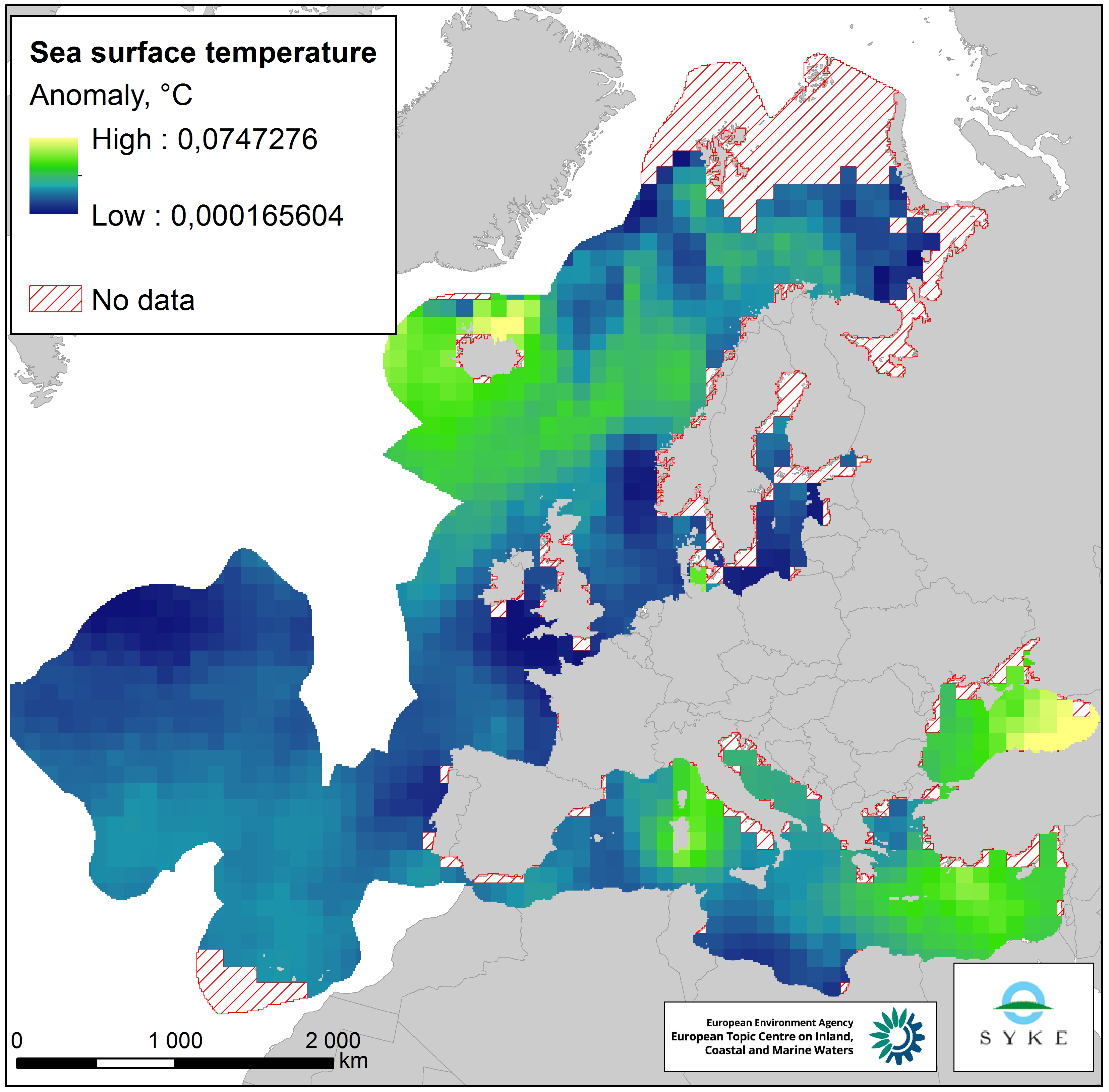
This raster dataset represents the Sea Surface Temperature (SST) anomalies, i.e. changes of sea temperatures, in the European Seas. The dataset is based on the map "Mean annual sea surface temperature trend in European seas" by Istituto Nazionale di Geofisica e Vulcanologia (INGV), which depicts the linear trend in sea surface temperature (in °C/yr) for the European seas over the past 25 years (1989-2013). Since all changes of sea temperatures can be considered to have an impact on the marine environment, the pressure layer includes absolute values of SST anomalies, i.e. negative/decreasing temperature trends were changed to positive values so that they represent a pressure. The original data was in a 1° grid format but was converted to a 100 km resolution, adapted to the EEA 10 km grid and clipped with the area of interest. This dataset has been prepared for the calculation of the combined effect index, produced for the ETC/ICM Report 4/2019 "Multiple pressures and their combined effects in Europe's seas" available on: https://www.eionet.europa.eu/etcs/etc-icm/etc-icm-report-4-2019-multiple-pressures-and-their-combined-effects-in-europes-seas-1.
-

'''This product has been archived''' '''DEFINITION''' The linear change of zonal mean subsurface temperature over the period 1993-2019 at each grid point (in depth and latitude) is evaluated to obtain a global mean depth-latitude plot of subsurface temperature trend, expressed in °C. The linear change is computed using the slope of the linear regression at each grid point scaled by the number of time steps (27 years, 1993-2019). A multi-product approach is used, meaning that the linear change is first computed for 5 different zonal mean temperature estimates. The average linear change is then computed, as well as the standard deviation between the five linear change computations. The evaluation method relies in the study of the consistency in between the 5 different estimates, which provides a qualitative estimate of the robustness of the indicator. See Mulet et al. (2018) for more details. '''CONTEXT''' Large-scale temperature variations in the upper layers are mainly related to the heat exchange with the atmosphere and surrounding oceanic regions, while the deeper ocean temperature in the main thermocline and below varies due to many dynamical forcing mechanisms (Bindoff et al., 2019). Together with ocean acidification and deoxygenation (IPCC, 2019), ocean warming can lead to dramatic changes in ecosystem assemblages, biodiversity, population extinctions, coral bleaching and infectious disease, change in behavior (including reproduction), as well as redistribution of habitat (e.g. Gattuso et al., 2015, Molinos et al., 2016, Ramirez et al., 2017). Ocean warming also intensifies tropical cyclones (Hoegh-Guldberg et al., 2018; Trenberth et al., 2018; Sun et al., 2017). '''CMEMS KEY FINDINGS''' The results show an overall ocean warming of the upper global ocean over the period 1993-2019, particularly in the upper 300m depth. In some areas, this warming signal reaches down to about 800m depth such as for example in the Southern Ocean south of 40°S. In other areas, the signal-to-noise ratio in the deeper ocean layers is less than two, i.e. the different products used for the ensemble mean show weak agreement. However, interannual-to-decadal fluctuations are superposed on the warming signal, and can interfere with the warming trend. For example, in the subpolar North Atlantic decadal variations such as the so called ‘cold event’ prevail (Dubois et al., 2018; Gourrion et al., 2018), and the cumulative trend over a quarter of a decade does not exceed twice the noise level below about 100m depth. Note: The key findings will be updated annually in November, in line with OMI evolutions. '''DOI (product):''' https://doi.org/10.48670/moi-00244
-
Annual time series of salmon escapement (2009-2014): • Time series of atlantic salmon escapement • Location and Long Term Average (LTA) of atlantic salmon escapement per Management Unit, that could be a river, basin district, a region or a whole country.
-
This product attempt to follow up on the sea level rise per stretch of coast of the North Atlantic, over past 10 years as follows: • Characterization of absolute sea level trend at annual resolution, along the coasts of EU Member States (including Outermost Regions), Canada, Faroes, Greenland, Iceland, Mexico, Morocco, Norway and USA; The stretchs or coast are defined by the administrative regions of the Atlantic Coast: • from NUTS3** administrative division for EU countries (see Eurostat), and • from GADM*** administrative divisions for non-EU countries. ** Third level of Nomenclature of Territorial Units for Statistics *** Global Administrative Areas For relative sea level trend for 10 years we extract the information from coastal tide gauge data available for each stretch of coast, if no tide gauge available there is a dat gap. The product is Provided in tabular form and as a map layer.
-
This product attempt to follow up on the sea level rise per stretch of coast of the North Atlantic, over past 10 years as follows: • Characterization of absolute sea level trend at annual resolution, along the coasts of EU Member States (including Outermost Regions), Canada, Faroes, Greenland, Iceland, Mexico, Morocco, Norway and USA; The stretchs or coast are defined by the administrative regions of the Atlantic Coast: • from NUTS3** administrative division for EU countries (see Eurostat), and • from GADM*** administrative divisions for non-EU countries. ** Third level of Nomenclature of Territorial Units for Statistics *** Global Administrative Areas For absolute sea level trend for 10 years we extract the information from grided satellite altimetry data and extrapolate it to the nearest strecth of coast. The product is Provided in tabular form and as a map layer.
-

'''This product has been archived''' For operationnal and online products, please visit https://marine.copernicus.eu '''DEFINITION''' The time series are derived from the regional chlorophyll reprocessed (REP) product as distributed by CMEMS. This dataset, derived from multi-sensor (SeaStar-SeaWiFS, AQUA-MODIS, NOAA20-VIIRS, NPP-VIIRS, Envisat-MERIS and Sentinel3A-OLCI) Rrs spectra produced by CNR using an in-house processing chain, is obtained by means of the Mediterranean Ocean Colour regional algorithms: an updated version of the MedOC4 (Case 1 (off-shore) waters, Volpe et al., 2019, with new coefficients) and AD4 (Case 2 (coastal) waters, Berthon and Zibordi, 2004). The processing chain and the techniques used for algorithms merging are detailed in Colella et al. (2021). Monthly regional mean values are calculated by performing the average of 2D monthly mean (weighted by pixel area) over the region of interest. The deseasonalized time series is obtained by applying the X-11 seasonal adjustment methodology on the original time series as described in Colella et al. (2016), and then the Mann-Kendall test (Mann, 1945; Kendall, 1975) and Sens’s method (Sen, 1968) are subsequently applied to obtain the magnitude of trend. '''CONTEXT''' Phytoplankton and chlorophyll concentration as a proxy for phytoplankton respond rapidly to changes in environmental conditions, such as light, temperature, nutrients and mixing (Colella et al. 2016). The character of the response depends on the nature of the change drivers, and ranges from seasonal cycles to decadal oscillations (Basterretxea et al. 2018). Therefore, it is of critical importance to monitor chlorophyll concentration at multiple temporal and spatial scales, in order to be able to separate potential long-term climate signals from natural variability in the short term. In particular, phytoplankton in the Mediterranean Sea is known to respond to climate variability associated with the North Atlantic Oscillation (NAO) and El Niño Southern Oscillation (ENSO) (Basterretxea et al. 2018, Colella et al. 2016). '''CMEMS KEY FINDINGS''' In the Mediterranean Sea, the trend average for the 1997-2020 period is slightly negative (-0.580.62% per year). Due to the change in processing techniques and chlorophyll retrieval, this trend estimate cannot be compared directly to those previously reported. The observations time series (in grey) shows minima values have been quite constant until 2015 and then there is a little decrease up to 2020, when an absolute minimum occurs with values lower than 0.04 mg m-3. Throughout the time series, maxima are variable year by year (with absolute maximum in 2015, >0.14 mg m-3), showing an evident reduction since 2016. In the last years of the series, the decrease of chlorophyll concentrations is also observed in the deseasonalized timeseries (in green) with a marked step in 2020. This attenuation of chlorophyll values in the last years results in an overall negative trend for the Mediterranean Sea. Note: The key findings will be updated annually in November, in line with OMI evolutions. '''DOI (product):''' https://doi.org/10.48670/moi-00259
-
Pentadal (5-year average) resolution time-series of bottom temperature for North Atlantic ocean area deeper than 1000m. Calculate the 5 year average bottom temperature at each point on the grid and then calculate the area weighted average.
-
This product attempt to follow up on the sea level rise per stretch of coast of the North Atlantic, over 50 years as follows: • Characterization of absolute sea level trend at annual resolution, along the coasts of EU Member States (including Outermost Regions), Canada, Faroes, Greenland, Iceland, Mexico, Morocco, Norway and USA; The stretchs or coast are defined by the administrative regions of the Atlantic Coast: • from NUTS3** administrative division for EU countries (see Eurostat), and • from GADM*** administrative divisions for non-EU countries. ** Third level of Nomenclature of Territorial Units for Statistics *** Global Administrative Areas For relative sea level trend for 50 years we extract the information from coastal tide gauges data available at each stretch of coast, if there is not a tide gauge there is a data gap. The product is Provided in tabular form and as a map layer.