Moving 6-year analysis of Water body chlorophyll-a in the NorthEast Atlantic for each season: - winter: January-March, - spring: April-June, - summer: July-September, - autumn: October-December. Every year of the time dimension corresponds to the 6-year centred average of each season. 6-year periods span from 1971/1976 until 2016/2021. Observation data span from 1971 to 2021. High-frequency observation trails were filtered to a 3h temporal resolution. Depth levels (IODE standard depths): [0.0, 5.0, 10.0, 20.0, 30.0, 40.0, 50.0, 75.0, 100.0, 125.0, 150.0, 200.0, 250.0, 300.0]. Data sources: observational data from SeaDataNet/EMODNet Chemistry Data Network. Descrption of DIVAnd analysis: the computation was done with DIVAnd (Data-Interpolating Variational Analysis in n dimensions), version 2.7.4, using GEBCO 30 sec topography for the spatial connectivity of water masses. The horizontal resolution of the produced DIVAnd maps is 0.1 degrees. Horizontal correlation length varies from 200km in open sea regions to 50km at the coast. Vertical correlation length is defined as twice the vertical resolution. Signal-to-noise ratio was fixed to 1 for vertical profiles and 0.1 for time series to account for the redundancy in the time series observations. A logarithmic transformation (DIVAnd.Anam.loglin) was applied to the data prior to the analysis to avoid unrealistic negative values. Background field: a vertically-filtered profile of the seasonal data mean value (including all years) is substracted from the data. Detrending of data: no, advection constraint applied: no. Units: mg/m3.

This visualization product displays beaches locations where the Marine Strategy Framework Directive (MSFD) monitoring protocol has been applied to collate data on macrolitter (> 2.5 cm). Reference lists associated with these protocols have been indicated with different colors in the map. EMODnet Chemistry included the collection of marine litter in its 3rd phase. Since the beginning of 2018, data of beach litter have been gathered and processed in the EMODnet Chemistry Marine Litter Database (MLDB). The harmonization of all the data has been the most challenging task considering the heterogeneity of the data sources, sampling protocols and reference lists used on a European scale. Preliminary processing were necessary to harmonize all the data: - Exclusion of OSPAR 1000 protocol: in order to follow the approach of OSPAR that it is not including these data anymore in the monitoring; - Selection of MSFD surveys only (exclusion of other monitoring, cleaning and research operations); - Exclusion of beaches without coordinates; - Some categories & some litter types like organic litter, small fragments (paraffin and wax; items > 2.5cm) and pollutants have been removed. The list of selected items is attached to this metadata. This list was created using EU Marine Beach Litter Baselines and EU Threshold Value for Macro Litter on Coastlines from JRC (these two documents are attached to this metadata). More information is available in the attached documents. Warning: the absence of data on the map doesn't necessarily mean that they don't exist, but that no information has been entered in the Marine Litter Database for this area.

This visualization product displays plastic bags density per trawl. EMODnet Chemistry included the collection of marine litter in its 3rd phase. Since the beginning of 2018, data of seafloor litter collected by international fish-trawl surveys have been gathered and processed in the EMODnet Chemistry Marine Litter Database (MLDB). The harmonization of all the data has been the most challenging task considering the heterogeneity of the data sources, sampling protocols (OSPAR and MEDITS protocols) and reference lists used on a European scale. Moreover, within the same protocol, different gear types are deployed during fishing bottom trawl surveys. In cases where the wingspread and/or number of items were unknown, data could not be used because these fields are needed to calculate the density. Data collected before 2011 are affected by this filter. When the distance reported in the data was null, it was calculated from: - the ground speed and the haul duration using this formula: Distance (km) = Haul duration (h) * Ground speed (km/h); - the trawl coordinates if the ground speed and the haul duration were not filled in. The swept area is calculated from the wingspread (which depends on the fishing gear type) and the distance trawled: Swept area (km²) = Distance (km) * Wingspread (km) Densities have been calculated on each trawl and year using the following computation: Density of plastic bags (number of items per km²) = ∑Number of plastic bags related items / Swept area (km²) Percentiles 50, 75, 95 & 99 have been calculated taking into account data for all years. The list of selected items for this product is attached to this metadata. Information on data processing and calculation is detailed in the attached methodology document. Warning: the absence of data on the map doesn't necessarily mean that they don't exist, but that no information has been entered in the Marine Litter Database for this area.

The drought index (DI) is computed using SMOS derived root zone soil moisture (RZSM) monthly fields. The concept is to consider 13 years of SMOS data (2010-2022). The RZSM monthly mean and max over the period is iused to compute a soil water deficit to remove seasonal variability. from teh soil water deficit a soil moisture drought index is computed .The range of values for SMDI lies between -4 to +4, with -4 representing extreme dry conditions and +4 representing extreme wet conditions.

This dataset comprises the global frequency, classification and distribution of marine heat waves (MHWs) from 1996-2020, in Chauhan et al. 2023 (https://doi.org/10.3389/fmars.2023.1177571). The classification was done based on their attributes and using different baselines. Daily SST values were extracted from the NOAA-OISST v2 high-resolution (0.25°) dataset from 1982-2020. MHWs were detected using the method presented by Hobday et al. 2016 (https://doi.org/10.1016/j.pocean.2015.12.014), and by using the 95th percentile of the accumulated temperature distribution to flag the extreme events. A shifting baseline of 8-year rolling period was selected between the years 1982-1996, since this period shows relatively stable maximum values of temperature across different ocean regions. The shifting baseline aims to account for the decadal changes of westerly winds, temperatures and ocean gyres circulations. The classification was done using the KMeans clustering algorithm to identify the relevant features of MHWs and classify them into separate groups based on feature similarities. This algorithm takes MHW features, namely duration, maximum intensity, rate onset and rate decline, as input vectors and applies clustering in the 4-dimensional feature space where each data point represents an MHW event. Note that all the MHWs features are standardized because unequal variances can put more weight on variables with smaller variances. This record comprehends the geospatial datasets of: Average number of MHW days per year (i.e., the sum of all MHW days divided by the total number of years, 1996-2020). Average cumulative intensity per year (i.e., the sum of cumulative intensity divided by the total number of years, 1996-2020). Total number of MHW events across the different periods averaged on the total number of years (1989-2020). The period 1982-1988 was only used as an initial baseline without calculating MHWs. Spatial distribution of three MHW categories: moderate MHWs, abrupt and Intense MHWs and extreme MHWs; displaying the total number of MHW days normalized by the number of years considered (i.e., 1989-2020). Distribution of Extreme MHWs across the different periods (A) 1989-1996, (B) 1997-2004, (C) 2005-2012, (D) 2013-2020. The relative frequency (γ) is a ratio of extreme MHWs in a specific period and all extreme MHWs in the same cluster for all periods.

This product displays for Lead, median values of the last 6 available years that have been measured per matrix and are present in EMODnet regional contaminants aggregated datasets, v2022. The median values ranges are derived from the following percentiles: 0-25%, 25-75%, 75-90%, >90%. Only "good data" are used, namely data with Quality Flag=1, 2, 6, Q (SeaDataNet Quality Flag schema). For water, only surface values are used (0-15 m), for sediment and biota data at all depths are used.

This product displays for Tributyltin, median values of the last 6 available years that have been measured per matrix and are present in EMODnet regional contaminants aggregated datasets, v2022. The median values ranges are derived from the following percentiles: 0-25%, 25-75%, 75-90%, >90%. Only "good data" are used, namely data with Quality Flag=1, 2, 6, Q (SeaDataNet Quality Flag schema). For water, only surface values are used (0-15 m), for sediment and biota data at all depths are used.

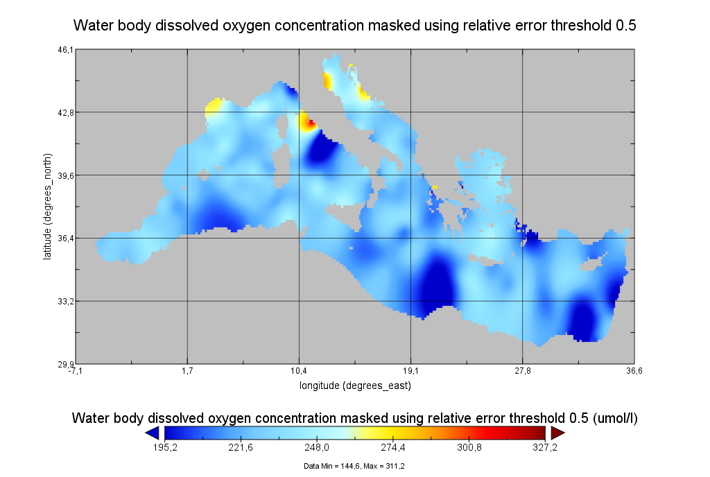
Moving 6-year analysis of Water body dissolved inorganic nitrogen (DIN) for each season: - winter: January-March, - spring: April-June, - summer: July-September, - autumn: October-December. Every year of the time dimension corresponds to the 6-year centered average of the season. 6-years periods span from 1990-1995 until 2017-2022. Data Sources: observational data from SeaDataNet/EMODNet Chemistry Data Network. Units: umol/l. Description of DIVA analysis: The computation was done with the DIVAnd (Data-Interpolating Variational Analysis in n dimensions), version 2.7.9, using GEBCO 30sec topography for the spatial connectivity of water masses. The horizontal resolution of the produced DIVAnd maps grids is dx=dy=0.125 degrees (around 13.5km and 10.9km accordingly). The vertical resolution is 21 depth levels: [0.,5.,10.,20.,30.,50.,75.,100., 125.,150.,200.,250.,300.,400.,500.,600.,700.,800.,900.,1000.,1100.]. The horizontal correlation length is 200km. The vertical correlation length (in meters) was set twices the vertical resolution: [10.,10.,20.,20.,40.,50.,50.,50.,50.,100.,100.,100.,200.,200.,200.,200.,200.,200.,200.,200.,200.]. Duplicates check was performed using the following criteria for space and time: dlon=0.001deg., dlat=0.001deg., ddepth=1m, dtime=1hour, dvalue=0.1. The error variance (epsilon2) was set equal to 1 for profiles and 10 for time series to reduce the influence of close data near the coasts. An anamorphosis transformation was applied to the data (function DIVAnd.Anam.loglin) to avoid unrealistic negative values: threshold value=200. A background analysis field was used for all years (1990-2022) with correlation length equal to 600km and error variance (epsilon2) equal to 20. Quality control of the observations was applied using the interpolated field (QCMETHOD=3). Residuals (differences between the observations and the analysis (interpolated linearly to the location of the observations) were calculated. Observations with residuals outside the minimum and maximum values of the 99% quantile were discarded from the analysis. Originators of Italian data sets-List of contributors: - Brunetti Fabio (OGS) - Cardin Vanessa, Bensi Manuel doi:10.6092/36728450-4296-4e6a-967d-d5b6da55f306 - Cardin Vanessa, Bensi Manuel, Ursella Laura, Siena Giuseppe doi:10.6092/f8e6d18e-f877-4aa5-a983-a03b06ccb987 - Cataletto Bruno (OGS) - Cinzia Comici Cinzia (OGS) - Civitarese Giuseppe (OGS) - DeVittor Cinzia (OGS) - Giani Michele (OGS) - Kovacevic Vedrana (OGS) - Mosetti Renzo (OGS) - Solidoro C.,Beran A.,Cataletto B.,Celussi M.,Cibic T.,Comici C.,Del Negro P.,De Vittor C.,Minocci M.,Monti M.,Fabbro C.,Falconi C.,Franzo A.,Libralato S.,Lipizer M.,Negussanti J.S.,Russel H.,Valli G., doi:10.6092/e5518899-b914-43b0-8139-023718aa63f5 - Celio Massimo (ARPA FVG) - Malaguti Antonella (ENEA) - Fonda Umani Serena (UNITS) - Bignami Francesco (ISAC/CNR) - Boldrini Alfredo (ISMAR/CNR) - Marini Mauro (ISMAR/CNR) - Miserocchi Stefano (ISMAR/CNR) - Zaccone Renata (IAMC/CNR) - Lavezza, R., Dubroca, L. F. C., Ludicone, D., Kress, N., Herut, B., Civitarese, G., Cruzado, A., Lefèvre, D.,Souvermezoglou, E., Yilmaz, A., Tugrul, S., and Ribera d'Alcala, M.: Compilation of quality controlled nutrient profiles from the Mediterranean Sea, doi:10.1594/PANGAEA.771907, 2011.

This product displays for Nickel, positions with percentages of all available data values per group of animals that are present in EMODnet regional contaminants aggregated datasets, v2022. The product displays positions for all available years.

EMODnet Chemistry aims to provide access to marine chemistry datasets and derived data products concerning eutrophication, acidity and contaminants. The importance of the selected substances and other parameters relates to the Marine Strategy Framework Directive (MSFD). This aggregated dataset contains all unrestricted EMODnet Chemistry data on eutrophication and acidity, and covers the Mediterranean Sea. Data were aggregated and quality controlled by the 'Hellenic Centre for Marine Research, Hellenic National Oceanographic Data Centre (HCMR/HNODC)' in Greece. ITS-90 water temperature and water body salinity variables have also been included ('as are') to complete the eutrophication and acidity data. If you use these variables for calculations, please refer to SeaDataNet for the quality flags: https://www.seadatanet.org/Products/Aggregated-datasets. Regional datasets concerning eutrophication and acidity are automatically harvested, and the resulting collections are aggregated and quality controlled using ODV Software and following a common methodology for all sea regions (https://doi.org/10.13120/8xm0-5m67). Parameter names are based on P35 vocabulary, which relates to EMODnet Chemistry aggregated parameter names and is available at: https://vocab.nerc.ac.uk/search_nvs/P35/. When not present in original data, water body nitrate plus nitrite was calculated by summing all nitrate and nitrite parameters. The same procedure was applied for water body dissolved inorganic nitrogen (DIN), which was calculated by summing all nitrate, nitrite, and ammonium parameters. Concentrations per unit mass were converted to a unit volume using a constant density of 1.025 kg/L. The aggregated dataset can also be downloaded as an ODV collection and spreadsheet, which is composed of a metadata header followed by tab separated values. This spreadsheet can be imported to ODV Software for visualisation (more information can be found at: https://www.seadatanet.org/Software/ODV).