 Catalogue PIGMA
*
Type of resources
Available actions
Topics
Keywords
Contact for the resource
Provided by
Years
Formats
Representation types
Update frequencies
status
Service types
Scale
Resolution
-
Auteur(s): Morel Hélène , Projet de reconversion de la grande halle en béton des anciens abattoirs de Bordeaux (quai de Paludate) en espace à dédié à la culture et aux loisirs
-
-

'''Short description:''' For the Mediterranean Sea - The product contains daily Level-3 sea surface wind with a 1km horizontal pixel spacing using Synthetic Aperture Radar (SAR) observations and their collocated European Centre for Medium-Range Weather Forecasts (ECMWF) model outputs. Products are processed homogeneously starting from the L2OCN products. '''DOI (product) :''' https://doi.org/10.48670/mds-00342
-
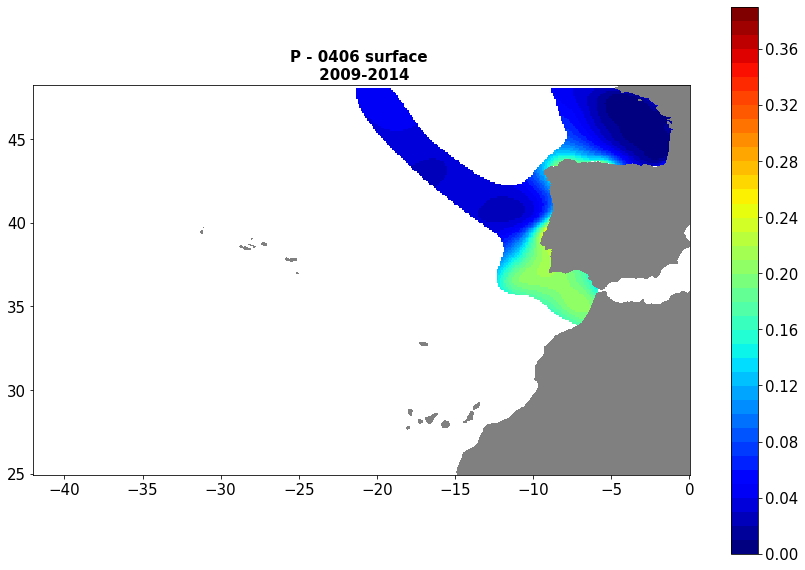
Moving 6-year analysis of Phosphate at Atlantic Sea for each season. - winter: January-March, - spring: April-June, - summer: July-September, - autumn: October-December Every year of the time dimension corresponds to the 6-year centred average of each season. 6-year periods span - from 1967-1972 until 2015-2020 (winter), - from 1960-1965 until 2015-2020 (spring), - from 1968-1973 until 2015-2020 (summer), - from 1961-1966 until 2015-2020 (autumn). Observational data span from 1960 to 2020. Depth range (IODE standard depths): -2000.0, -1750, -1500.0, -1400.0, -1300.0, -1200.0, -1100.0, -1000.0, -900.0, -800.0, -700.0, -600.0, -500.0, -400.0, -300.0, -250.0, -200.0, -150.0, -125.0, -100.0, -75.0, -50.0,-40.0, -30.0, -20.0, -10.0, -5.0, -0.0 Data Sources: observational data from SeaDataNet/EMODNet Chemistry Data Network. Description of DIVA analysis: Geostatistical data analysis by DIVA (Data-Interpolating Variational Analysis) tool. GEBCO 1min topography is used for the contouring preparation. Analyzed filed masked using relative error threshold 0.3 and 0.5 DIVA settings. Correlation length was optimized and filtered vertically and a seasonally-averaged profile was used. Signal to noise ratio was fixed to 1. Logarithmic transformation applied to the data prior to the analysis. Background field: the data mean value is subtracted from the data. Detrending of data: no, Advection constraint applied: no. Units: umol/l
-

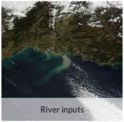
As part of the European Horizon Europe FOCCUS project (https://foccus-project.eu/), the metadata inventory of European coastal platforms has been extracted. The inventory was based on the following History and Latest products, downloaded from the CMEMS website (https://marine.copernicus.eu/fr/acces-donnees) at: 1) Global Ocean-In-Situ Near-Real-Time Observation, 2) Atlantic Iberian Biscay Irish Ocean-In-Situ Near Real Time Observations, 3) Mediterranean Sea-In-Situ Near Real Time Observations, 4) Atlantic-European North West Shelf-Ocean In-Situ Near Real Time Observations. To carry out this inventory, it was decided to target only coastal platforms, located less than 200km from the coast and at a depth of less than 400m. For mobile platforms, it was also decided to focus only on the first position in the file. This data must be located within 200 km of the coast and at a depth of less than 400 m. In this inventory, FerryBox platforms have all been considered as coastal platforms. The following platforms were extracted from the products: BO (Bottles), CT (CTD), DB (Drifting Buoys), FB (Ferry Box), GL (Gliders), HF (High Frequency Radar), MO (Mooring), PF (Profiling Float), TG (Tide Gauge) and XB (XBT). Once the metadata had been extracted from the files, duplicates were removed (files with the same names). Duplicate platforms of type _TS_ and _WS_ were merged (date and parameters). Latest‘ files have been merged with ’History" files. Missing metadata have been replaced in the Excel file by ‘Missing Data’. Some old dates were also revised by hand because they had been badly extracted, as well as some institution names that included special characters. Platforms located on estuaries/rivers/lakes/ponds have also been removed by hand. This inventory identified a total of 10,479 coastal platforms.
-

-
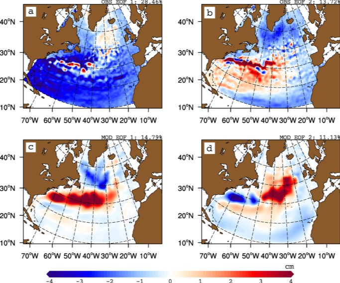
The gyre index constructed here from satellite altimetry is related to core aspects of the North Atlantic subpolar gyre, meridional overturning circulation, hydrographic properties in the Atlantic inflows toward the Arctic, and in marine ecosystems in the northeast Atlantic Ocean. The data series spans the period January 1993 to September 2018. Data description: Monthly gyre index from January 1993 until September 2018. The data is provided in one comma separated value (csv) file with the following entries on each row: year, month, index value. The index is normalized, i.e. it has a zero mean and unit standard deviation. Positive (negative) gyre index reflects stronger (weaker) than average surface circulation of the North Atlantic subpolar gyre.
-

-
Auteur(s): Combe Caroline , Réflexion sur la conception de l'étape contemporaine du pèlerin sur le chemin de Saint-Jacques-de-Compostelle. Développement d'un projet d'étape à Roquefort, dans les Landes : insertion dans la ville, cohabitation de fonctions laïques et religieuses, transcription spatiale d'une symbolique liée au sacré.
-