 Catalogue PIGMA
2020
Type of resources
Available actions
Topics
Keywords
Contact for the resource
Provided by
Years
Formats
Representation types
Update frequencies
status
Service types
Scale
Resolution
-
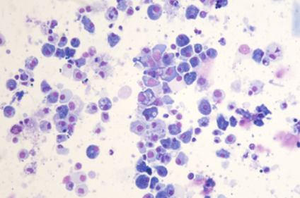
scRNA-seq reads from a Pacific oyster (Crassostrea gigas) hemocyte preparation. Hemocytes were isolated from a unique immunologically naive animal (Ifremer Standardized Animal, 18 months) and single-cell drop-seq technology was applied to 3,000 individual hemocytes.
-
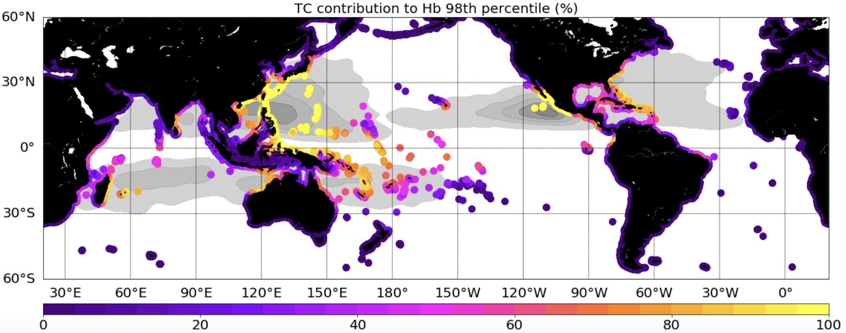
This dataset provides extreme waves (Hs: significant wave height, Hb:breaking wave height, a proxy of the wave energy flux) simulated with the WWIII model, and extracted along global coastlines. Two simulations, including or not Tropical Cyclones (TCs) in the forcing wind field, are provided.
-
Périmètre de la CAPB
-
Maisons de la communauté
-
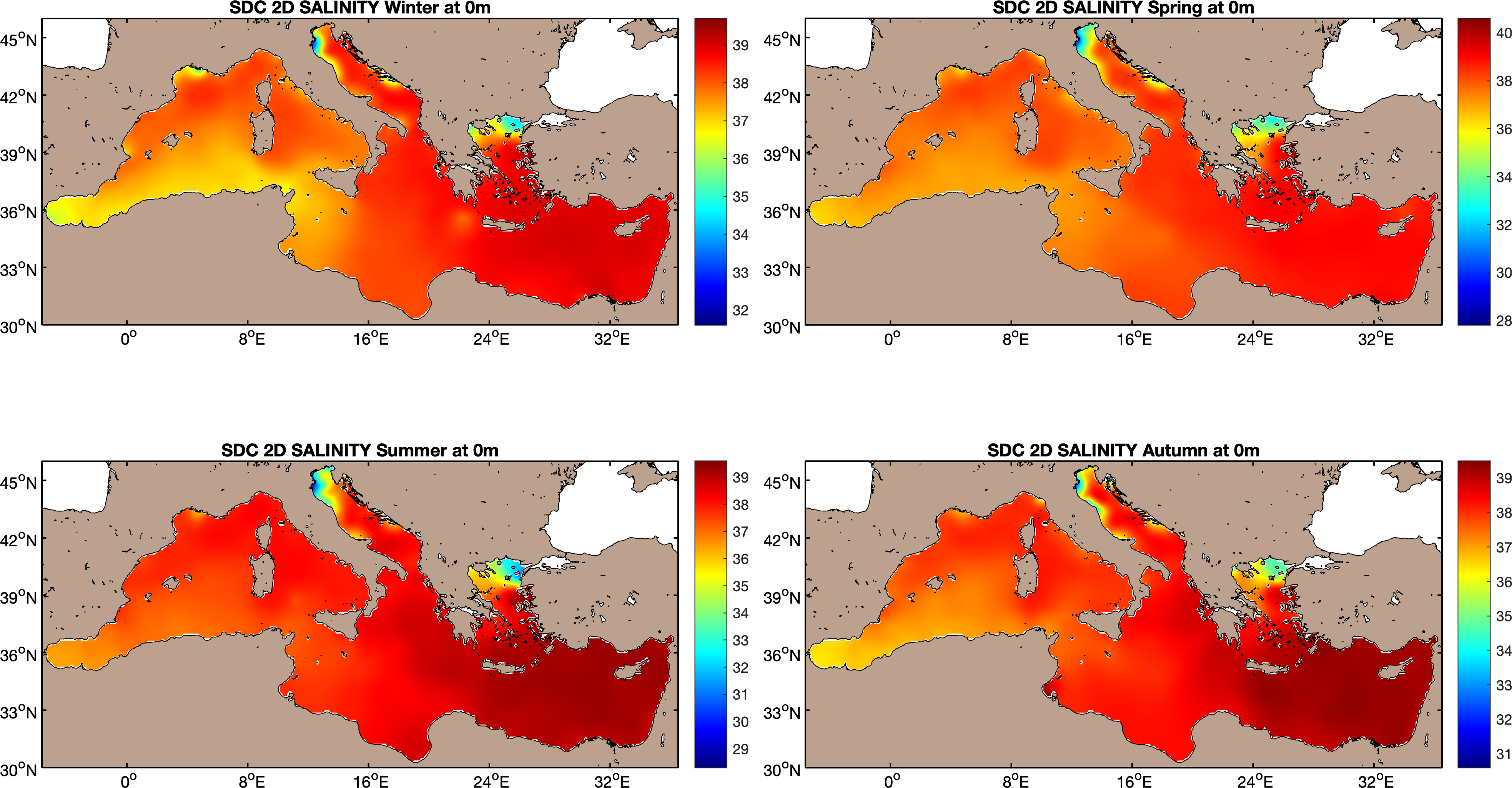
The SDC_MED_CLIM_TS_V2 product contains Temperature and Salinity Climatologies for Mediterranean Sea: monthly and seasonal fields for time periods 1955-2018, 1955-1984 and 1985-2018 and seasonal fields for 6 decades covering the time period 1955 to 2018. The climatic fields were computed from an integrated Mediterranean Sea data set that combines data extracted from SeaDataNet infrastructure (SDC_MED_DATA_TS_V2, https://doi.org/10.12770/2a2aa0c5-4054-4a62-a18b-3835b304fe64) and Coriolis Ocean Dataset for Reanalysis (CORA5.2) distributed by the Copernicus Marine Service (INSITU_GLO_TS_REP_OBSERVATIONS_013_001_b). The computation was done with the DIVAnd (Data-Interpolating Variational Analysis), version 2.4.0.
-
The SDC_GLO_CLIM_TS_V2 product is an improved version of SDC_GLO_CLIM_TS_V1 and contains two different monthly climatologies for temperature and salinity from the World Ocean Data 2018 (WOD-18) database. Along with the basic quality control flags from the WOD-18, an additional quality Control named Nonlinear Quality Control (NQC) is applied. The first climatology, V2_1, considers temperature and salinity profiles from Conductivity Depth Temperature (CTD), Ocean station data (OSD) and Moored buoy data (MRB) along with Profiling Floats (PFL) from 1900 to 2017. The second climatology, V2_2, utilizes only PFL data from 2003 to 2017. V2_1 considers 44 layers from surface to 6000 m while V2_2 only 34 from 0 to 2000 m. The gridded fields are computed using DIVAnd (Data Interpolating Variational Analysis) version 2.3.1. For data access, please register at http://www.marine-id.org/.
-
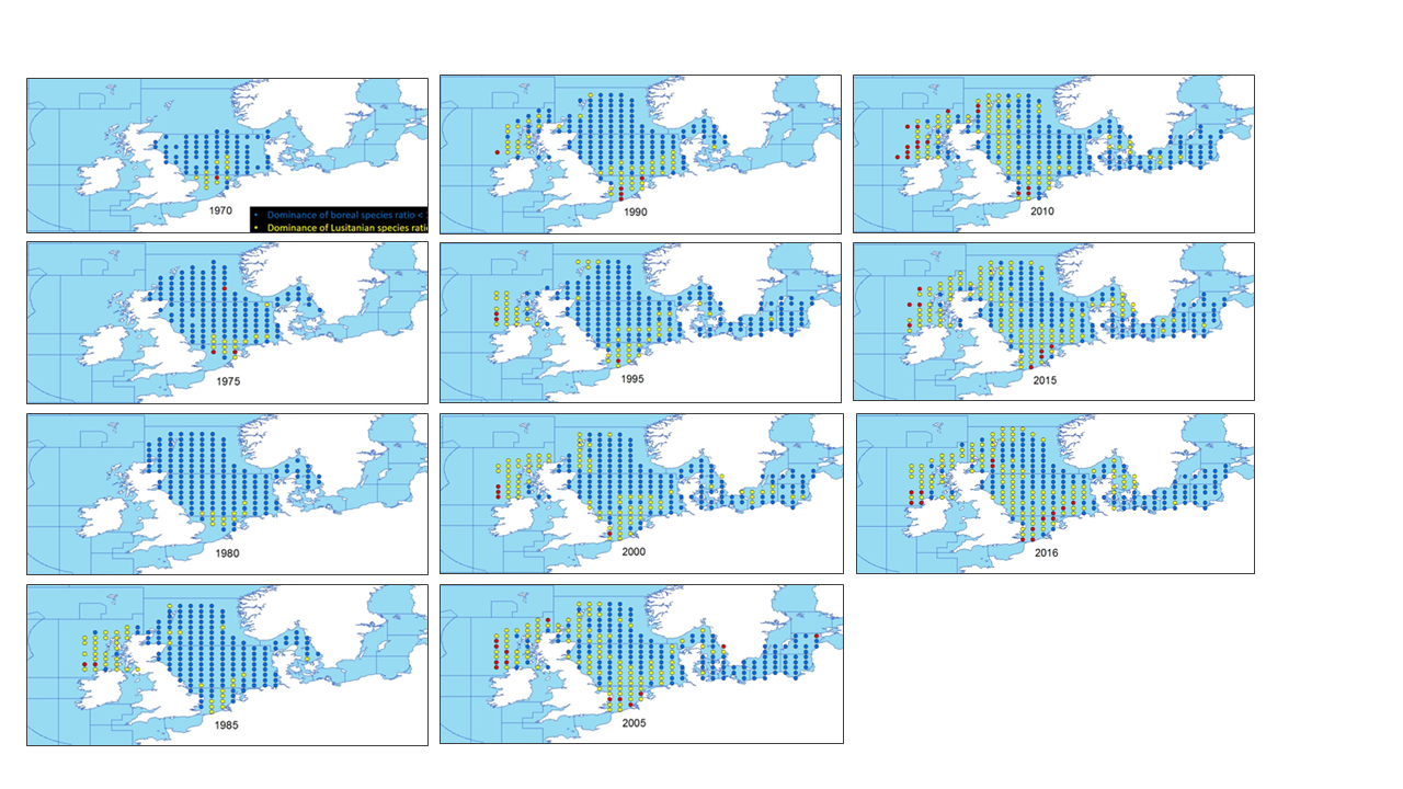
This metadata describes the ICES data on the temporal development of the Lusitanian/Boreal species ratio in the period from 19657 to 2016. Key message: The ratio between the number of Lusitanian (warm-favouring) and Boreal (cool-favouring) species are significantly increasing in several North-East Atlantic marine areas whereas there is no significant changes in all the southern areas. Changes in ratios are most apparent in the North Sea, Irish Sea and West of Scotland. Furthermore, it seems that Lusitanian species have not spread in all northward directions, but have followed two particular routes, through the English Channel and north around Scotland Blue dots indicates L/B ratios below 1 (dominance of Boreal species) Yellow dots indicates L/B ratios >=1 and <2 (dominance of Lusitanian species) Red dots indicates L/B ratios >=2 (high dominance of Lusitanian species) The dataset is derived from the ICES data portal 'DATRAS' (the Database of Trawl Surveys). DATRAS is an online database of trawl surveys with access to standard data products. DATRAS stores data collected primarily from bottom trawl fish surveys coordinated by ICES expert groups. The survey data are covering the Baltic Sea, Skagerrak, Kattegat, North Sea, English Channel, Celtic Sea, Irish Sea, Bay of Biscay and the eastern Atlantic from the Shetlands to Gibraltar. At present, there are more than 56 years of continuous time series data in DATRAS, and survey data are continuously updated by national institutions. The dataset has been used in the EEA Indicator "Changes in fish distribution in European seas" https://www.eea.europa.eu/data-and-maps/indicators/fish-distribution-shifts/assessment-1. The dataset has been used for this static map: https://www.eea.europa.eu/en/analysis/indicators/changes-in-fish-distribution-in/temporal-development-of-the-ratio
-

This study gathers multi-year environmental sequencing datasets generated within the French ROME pilot observatory network. It includes eDNA metabarcoding and RNA-based analyses from water samples, oyster tissues, and viral fractions collected across four French estuarine ecosystems between 2020 and 2023, supporting integrated monitoring of coastal microbiomes and microbial hazards.
-
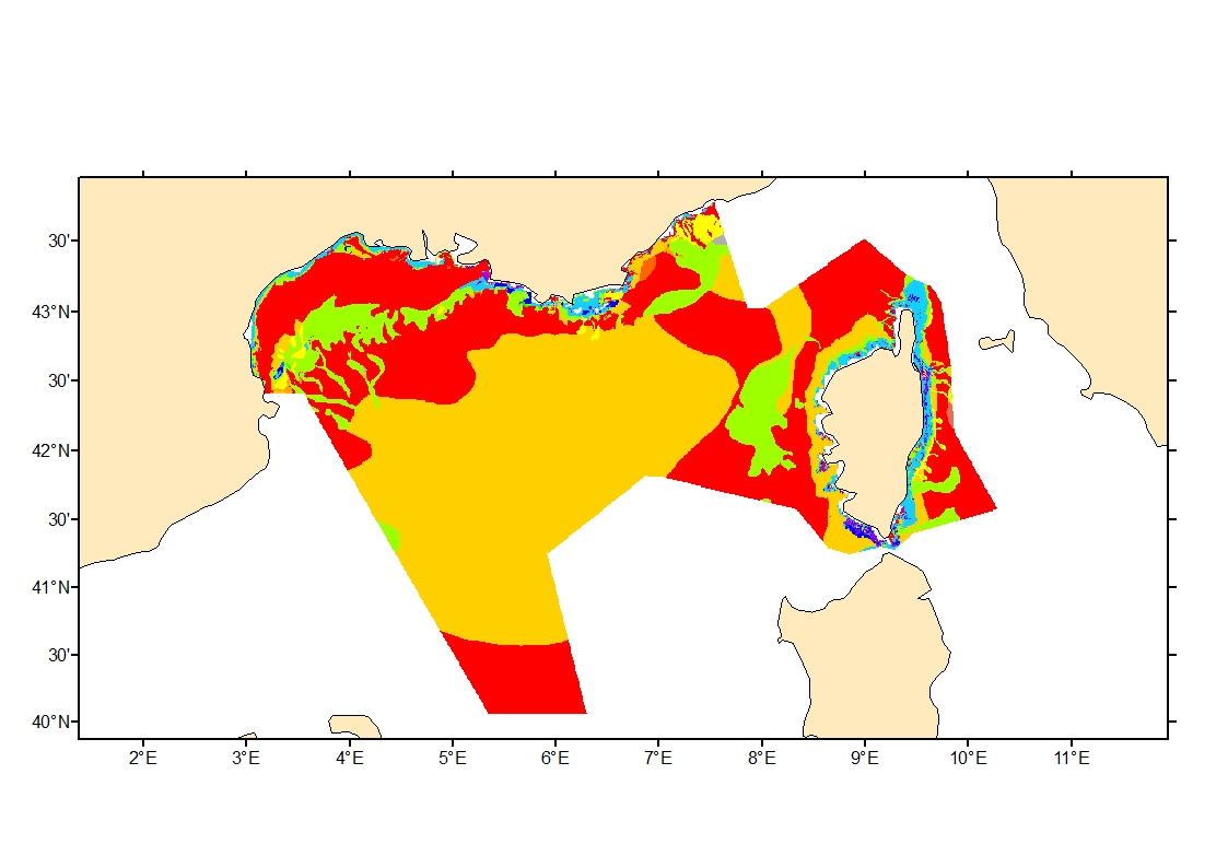
Sediment average grain size in French Mediterranean waters was generated from sediment categories. This rough granulometry estimate may be used for habitat models at meso- and large scale.
-
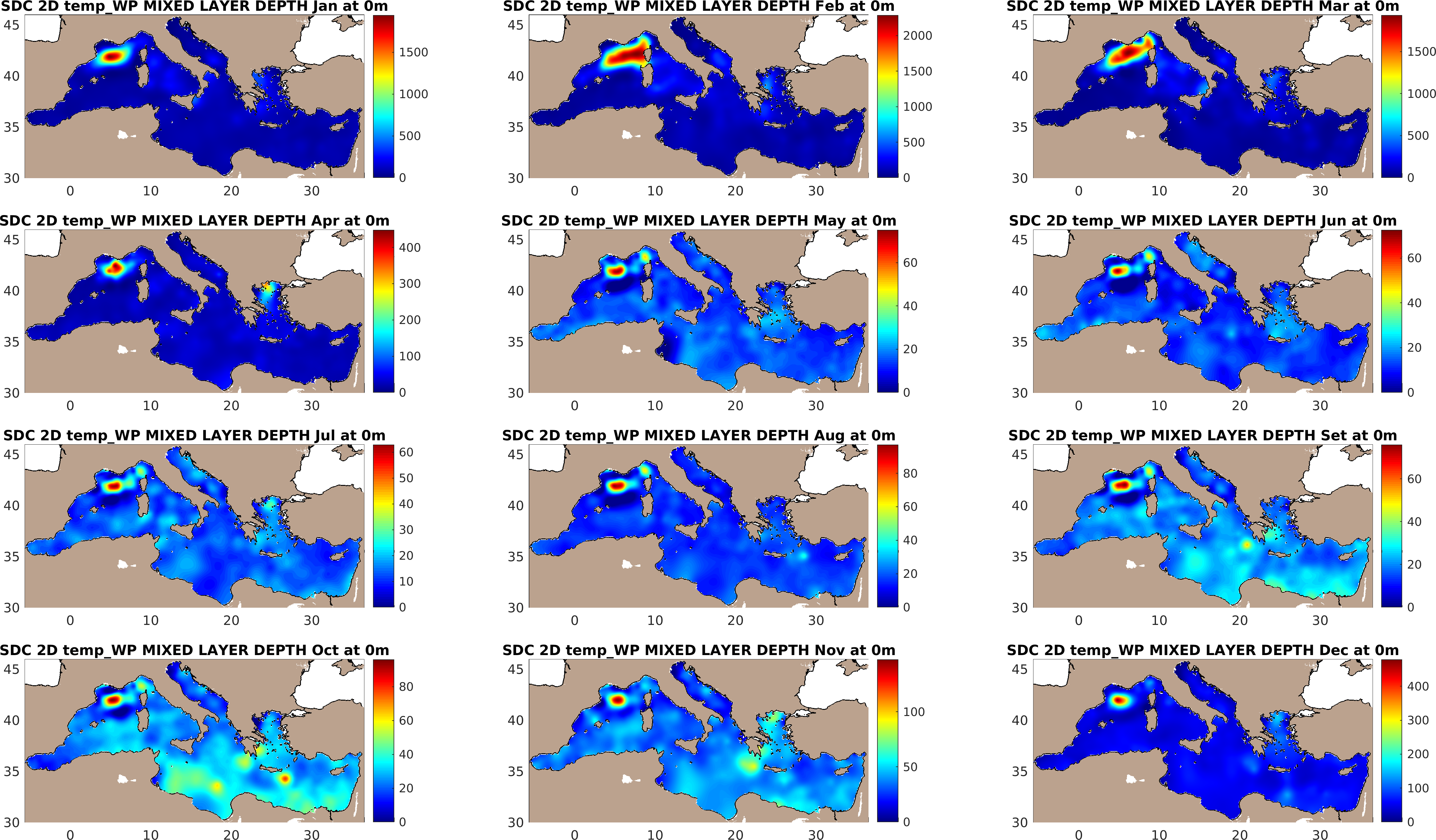
The SDC_MED_DP1 consists of Mixed Layer Depth (MLD) monthly climatology at 1/8 of degree for the Mediterranean Sea computed from an integrated dataset of collocated temperature and salinity profiles which combines data extracted from SeaDataNet infrastructure (SDC_MED_DATA_TS_V1, https://doi.org/10.12770/2698a37e-c78b-4f78-be0b-ec536c4cb4b3) and the Coriolis Ocean Dataset for Reanalysis (CORA), version 5.2 (https://archimer.ifremer.fr/doc/00595/70726/). The products comprehends three versions of MLD climatology over the 1955-2017 time period obtained computing the MLD from three different methods. A MLD climatology for the time span 1987-2017 computed with the fixed density criteria is also available. The analysis was done with the DIVAnd (Data-Interpolating Variational Analysis in n dimensions), version 2.6.1.