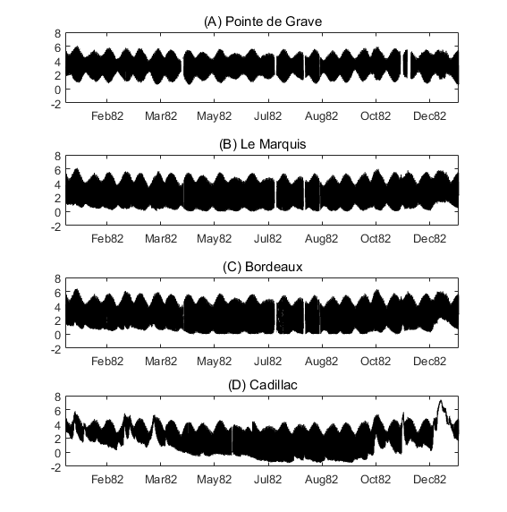
Times series of water level at four stations of the Gironde Estuary (Pointe de Grave, Le Marquis, Bordeaux and Cadillac) for the the years 1953, 1971, 1982, 1994, 2005 and 2014. The dataset includes all of the time seris used in the publication: To what extent multidecadal changes in morphology and fluvial discharge impact tide in a convergent (turbid) tidal river (2018), Journal of Geophysical Research: Oceans.

Global mean sea level is an integral of changes occurring in the climate system in response to unforced climate variability as well as natural and anthropogenic forcing factors. Its temporal evolution allows detecting changes (e.g., acceleration) in one or more components. Study of the sea level budget provides constraints on missing or poorly known contributions, such as the unsurveyed deep ocean or the still uncertain land water component. In the context of the World Climate Research Programme Grand Challenge entitled “Regional Sea Level and Coastal Impacts”, an international effort involving the sea level community worldwide has been recently initiated with the objective of assessing the various data sets used to estimate components of the sea level budget during the altimetry era (1993 to present). These data sets are based on the combination of a broad range of space-based and in situ observations, model estimates and algorithms. Evaluating their quality, quantifying uncertainties and identifying sources of discrepancies between component estimates is extremely useful for various applications in climate research. This effort involves several tens of scientists from about sixty research teams/institutions worldwide (www.wcrp-climate.org/grand-challenges/gc-sea-level). The results presented in this paper are a synthesis of the first assessment performed during 2017-2018. We present estimates of the altimetry-based global mean sea level (average rate of 3.1 +/- 0.3 mm/yr and acceleration of 0.1 mm/yr2 over 1993-present), as well as of the different components of the sea level budget. We further examine closure of the sea level budget, comparing the observed global mean sea level with the sum of components. Ocean thermal expansion, glaciers, Greenland and Antarctica contribute by 42%, 21%, 15% and 8% to the global mean sea level over the 1993-present. We also study the sea level budget over 2005-present, using GRACE-based ocean mass estimates instead of sum of individual mass components. Results show closure of the sea level budget within 0.3 mm/yr. Substantial uncertainty remains for the land water storage component, as shown in examining individual mass contributions to sea level.

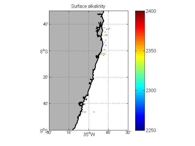
Inorganic carbon and alkalinity measurements (in micromoles/kg) along the coast of Brazil, 2013-2015.  

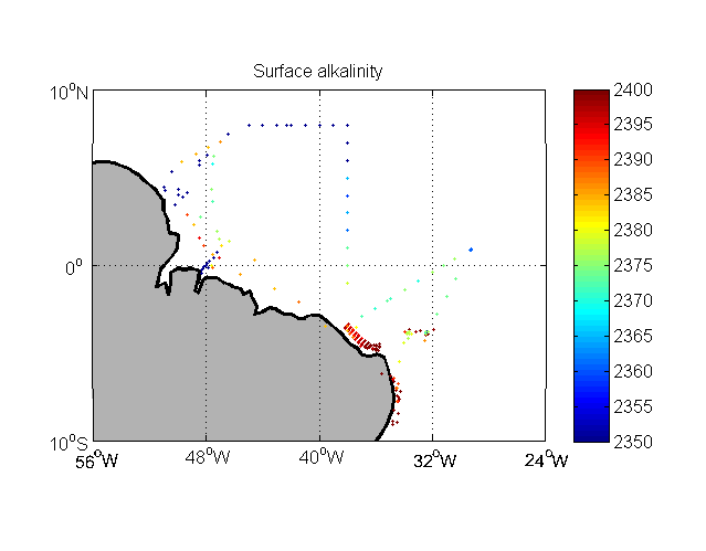
Inorganic carbon and alkalinity measurements (in micromoles/kg) from Brazilian cruises in the Western Tropical Atlantic.

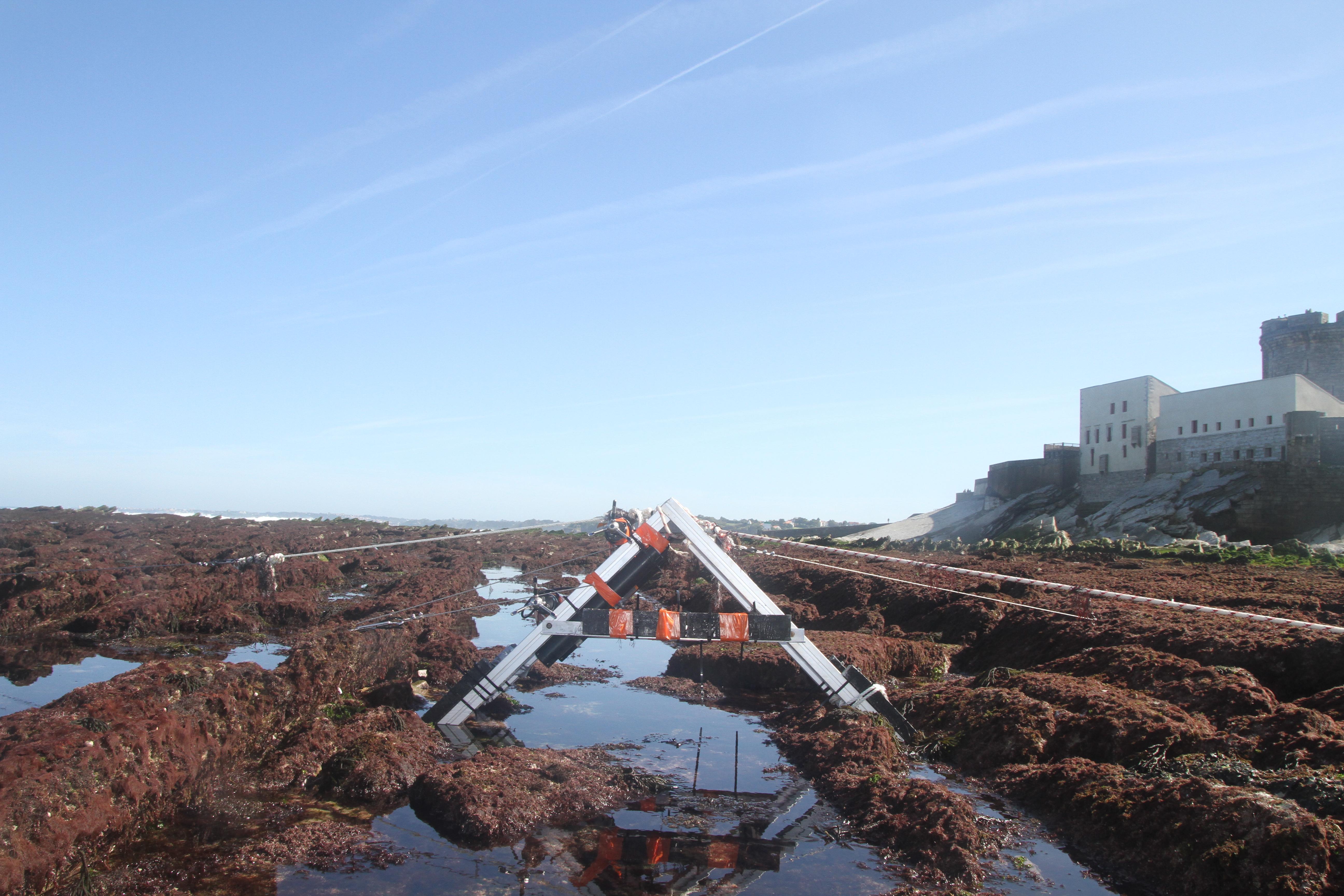
The database displays the field measurements recover during a one-week experiment in October 2021 on the Socoa's rocky platform, France. The general objective of the study was to evaluate the momentum balance over the rocky platform, in particular to quantifiy the combined effect of high seabed roughness and waves on the coupling between circulation, wave force and mean water level. The analysis is performed along a single cross-shore transect.  The data include: - the cross-shore bathymetric profile - the time-series of integrated wave parameters, local mean water depth and wave-averaged currents over successive 30-min bursts - the depth- and wave-averaged momentum fluxes following the formulation proposed by Smith 2006 and Bruneau et al. 2011. The fluxes are median values obtained over significant wave height to depth ratio bins

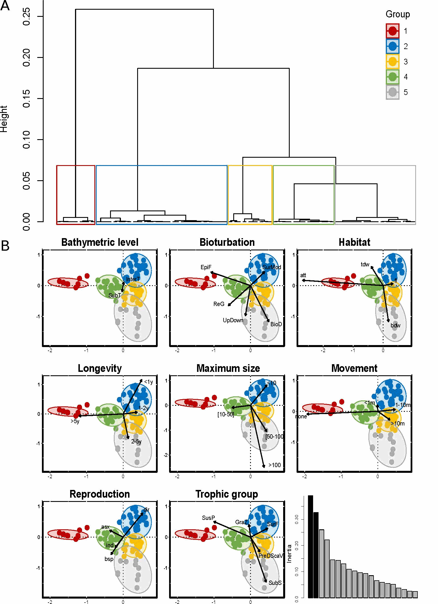
Reef-building species are recognized as having an important ecological role and as generally enhancing the diversity of benthic organisms in marine habitats.  However, although these ecosystem engineers have a facilitating role for some species, they may exclude or compete with others. The honeycomb worm Sabellaria alveolata (Linnaeus, 1767) is an important foundation species, commonly found from northwest Ireland to northern Mauritania (Curd et al., 2020), whose reef structures increase the physical complexity of the marine benthos, supporting high levels of biodiversity. Local patterns and regional differences in taxonomic and functional diversity were examined in honeycomb worm reefs from ten sites along the northeastern Atlantic to explore variation in diversity across biogeographic regions and the potential effects of environmental drivers. To characterize the functional diversity at each site, a biological trait analysis (BTA) was conducted (Statzner et al., 1994). Here we present the functional trait database used for the benthic macrofauna found to live in association with honeycomb worm reefs. Eight biological traits (divided into 32 modalities) were selected (Table 1), providing information linked to the ecological functions performed by the associated macrofauna. The selected traits provide information on: (i) resource use and availability (by the trophic group of species, e.g. Thrush et al. 2006); (ii) secondary production and the amount of energy and organic matter (OM) produced based on the life cycle of the organisms (including longevity, maximum size and mode of reproduction, e.g. (Cusson and Bourget, 2005; Thrush et al., 2006) and; (iii) the behavior of the species in general [i.e. how these species occupy the environment and contribute to biogeochemical fluxes through habitat, movement, and bioturbation activity at different bathymetric levels, e.g. (Solan et al., 2004; Thrush et al., 2006; Queirós et al., 2013). Species were scored for each trait modality based on their affinity using a fuzzy coding approach (Chevenet et al., 1994), where multiple modalities can be attributed to a species if appropriate, and allowed for the incorporation of intraspecific variability in trait expression. The information concerning polychaetes was derived primarily from Fauchald et al (1979) and Jumars et al (2015). Information on other taxonomic groups was obtained either from databases of biological traits (www.marlin.ac.uk/biotic) or publications (Naylor, 1972; King, 1974; Caine, 1977; Lincoln, 1979; Holdich and Jones, 1983; Smaldon et al., 1993; Ingle, 1996; San Martín, 2003; Southward, 2008; Gil, 2011; Leblanc et al., 2011; Rumbold et al., 2012; San Martín and Worsfold, 2015; Jones et al., 2018). Map indicating the locations of the 10 study sites in the UK, France and Portugal within the four biogeographic provinces defined by Dinter (2001). (All sites were sampled in 8 different stations, except for UK4 where 5 stations were sampled).

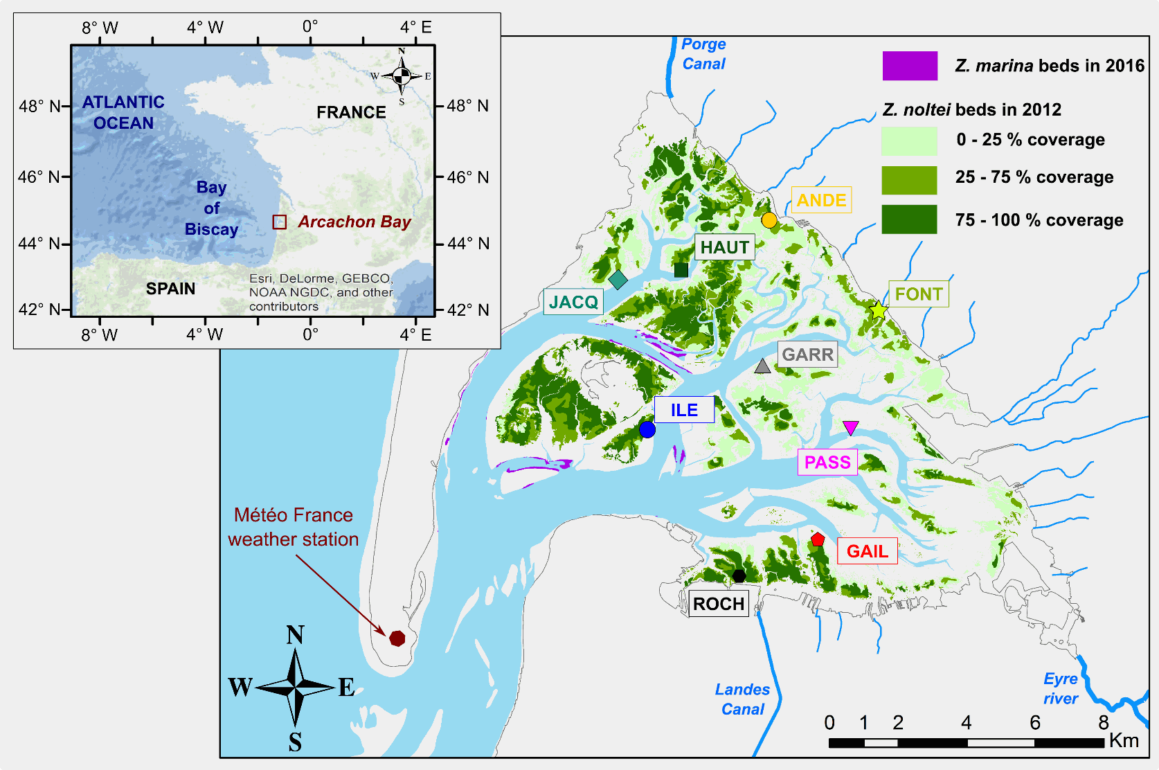
The ReZoEnv field campaign was conducted at 9 sites distributed within contrasted seagrass (Zostera notlei) meadows in the Arcachon Bay. This multi-parameter survey was conducted during one year (November 2015 – November 2016). Water levels, temperature and light were recorded every 10 minutes. While bed sediment characteristics (granulometry, water content, organic matter content), seagrass characteristics (coverage, biometry, chlorophyll and CNP content) were measured monthly. Additionally, wind-wave parameters were obtained from high frequency pressure sensor at 4 sites, every 20 minutes. List of sites : - ANDE : 44.745091 N, 1.121366 O - FONT : 44.722631 N, 1.080133 O - GAIL : 44.662573 N, 1.099575 O - GARR : 44.705132 N, 1.121562 O - HAUT : 44.729331 N, 1.15608 O - ILE : 44.683117 N, 1.162716 O - JACQ : 44.724563 N, 1.181109 O - PASS : 44.689927 N, 1.089491 O - ROCH : 44.648529 N, 1.127736 O

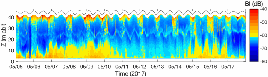
In the framework of the ANR AMORAD project, the METEOR cruises (Grasso, 2017) aimed at deploying the ‘Gironde Estuary Mouth MEasurement Stations’ (GEMMES) to measure hydrodynamics and sediment dynamics at the mouth of the Gironde Estuary and on the West Gironde Mud Patch (SW France, Bay of Biscay). Measurements were carried out between November 2016 and December 2017: i) from a buoy station around 20-m water depth (GEMMES-20), collecting sub-surface data of temperature, salinity and turbidity; and ii) a benthic station around 40-m water depth (GEMMES-40), collecting data of current velocity and turbidity. Bottom and surface water samples were regularly collected to calibrate turbidity measurements to SPM concentrations.

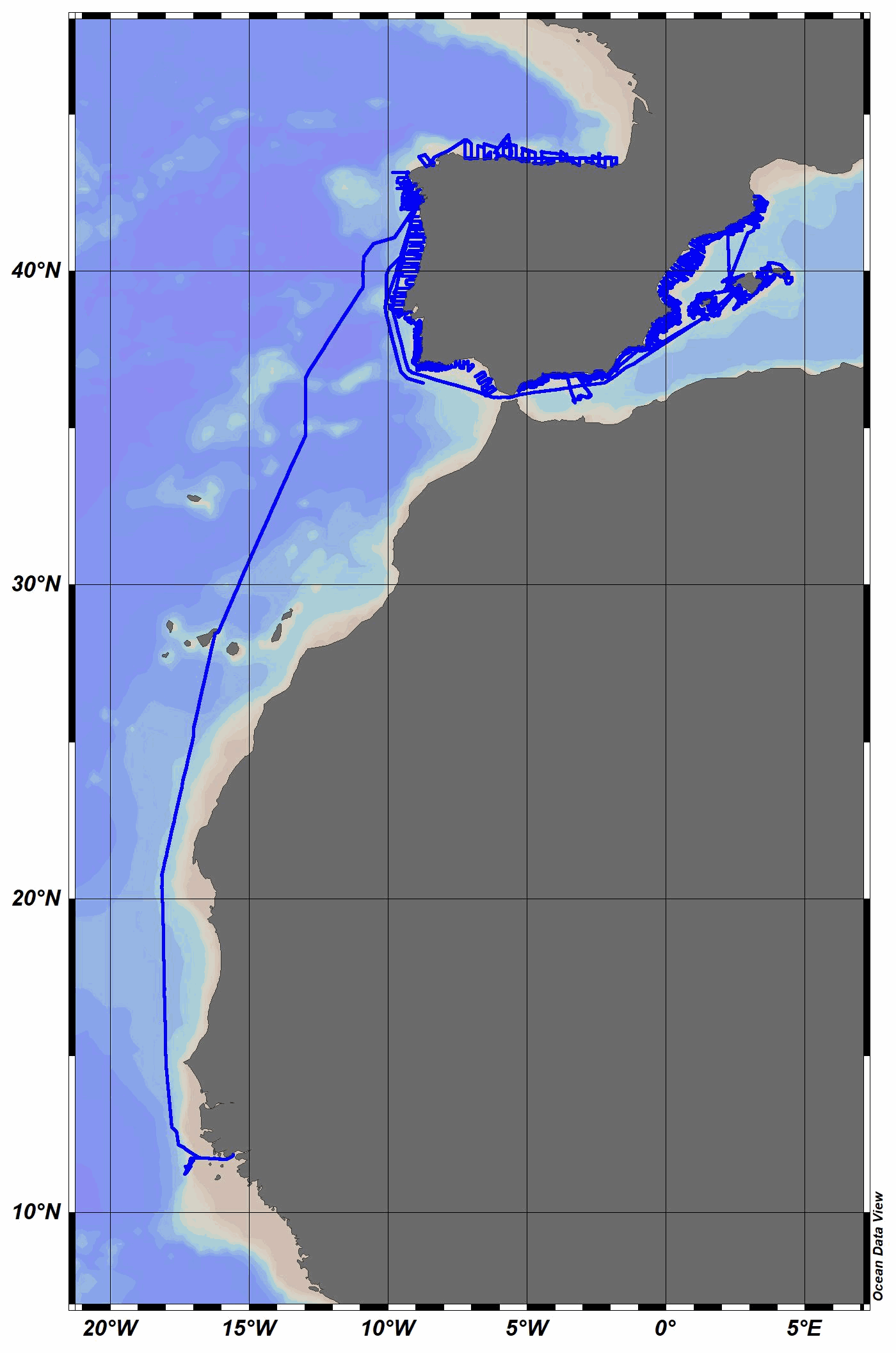
The R/V Miguel Oliver was built in 2007 for scientific fisheries assessment and oceanographic research purposes. Owned by the Spanish General Secretariat of Fisheries, it mainly operates around the Iberian Peninsula and Canary Islands waters. Equipped with an automatic weather station, collected data are daily sent to the Spanish Institute of Oceanography (IEO) Data Center / National Oceanographic Data Center (NODC) for delayed-mode quality control and long-term archive and dissemination. Recently, a semi-automatic process has been used to perform quality control and data assessment. The quality controlled data have been stored in MEDAR/MEDATLAS format, and the corresponding quality flag has been added to each individual measurement. This facilitates their reuse for different purposes, from climatology or academic studies to industrial sector needs, among others. In 2023, air temperature, relative humidity, wind speed and direction and solar radiation were collected.

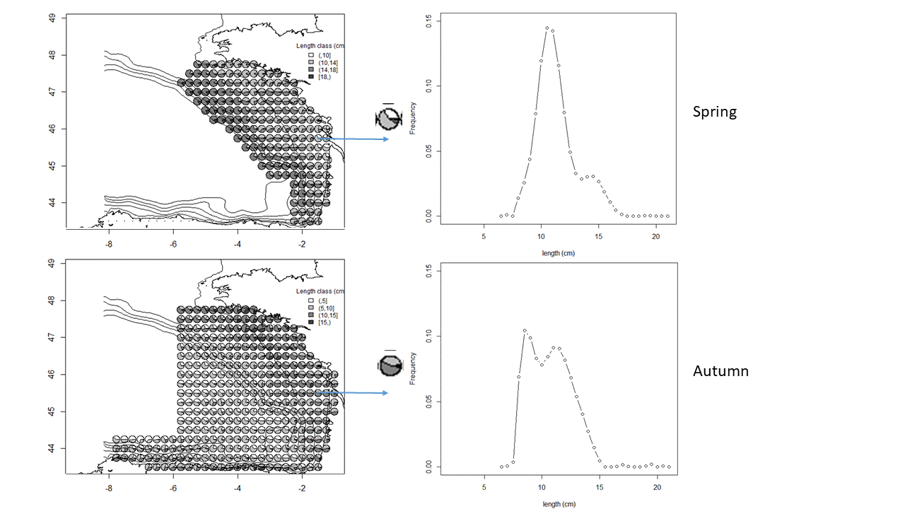
The anchovy (Engraulis encrasicolus) and sardine (Sardina pilchardus) populations in the Bay of Biscay are jointly surveyed each year in May since 2000 and in September since 2003 by means of acoustic surveys. The integrated survey PELGAS (Doray et al., 2018) is run in May by France and covers the French shelf of the Bay of Biscay. Its objectives are to monitor the Bay of Biscay pelagic ecosystem in springtime and assess the biomass of its small pelagic fish species, including sardine and anchovy. Amongst many information on the ecosystem, the survey PELGAS provides knowledge on the adults of anchovy and sardine during their spawning in spring. The survey JUVENA (Boyra et al., 2013) is run in September by Spain. It has a larger spatial coverage than PELGAS, including part of the Spanish coast and open ocean outside the shelf because it targets juvenile anchovy. It also provides knowledge on sardine as well as other pelagic species. Both surveys are coordinated by the ICES Working Group on Acoustic and Egg Surveys for Small Pelagic Fish (WGACEGG), together with other pelagic surveys in ICES areas 7, 8 and 9. Survey protocoles are detailed in Doray et al. (2021). Briefly, fish backscatter data are recorded along the survey transect lines and pelagic trawl hauls are undertaken opportunistically to identify the echotraces to species and collect fish samples for biometric data. The trawl haul catches have provided the anchovy and sardine length data, from which the maps presented here are derived. At each trawl haul, the catch is sorted by species and weighted. A subsample by species is measured to estimate the species’ length distribution. The four maps presented here correspond to the average maps of anchovy and sardine length distributions in May and September, derived from the PELGAS and JUVENA trawl haul data series. The maps were obtained by kriging, following the procedure explained in Petitgas et al. (2011) for mapping functions instead of variables. For each species, the experimental length distribution at each haul was fitted by a linear combination of Legendre polynomials, the coefficients of which were co-kriged. The number of polynomials varied from 15 to 22 depending on the survey and species, with a higher number for sardine and in autumn. The length histogram at each grid node was then deduced from the mapped coefficients. When the length distribution at a given haul was estimated with less than 40 individual fish, the haul was not taken into account for mapping. This threshold defined presence and absence of the species in the haul data sets. The trawl hauls from 2000 to 2019 were pooled for the PELGAS series (1965 stations) and from 2003 to 2020 for JUVENA (852 stations). The mapping was performed on the same grid for both PELGAS and JUVENA and both species, and with similar moving kriging neighbourhoods. The grid has a mesh size of 0.25 x 0.25 decimal degree square. In addition to mapping the length distribution, presence/absence was mapped for each species by ordinary kriging on the same grid and with the same neighbourhoods as previously. The computations were performed in R (version 4.0.5) with the RGeostats package (version 13.0.1) freely available at http://rgeostats.free.fr. The map data files comprise for each species the following information: the geographical coordinates of the grid points, the probability of presence and the probability of each length class of width 0.5 cm ranging from 2.5 to 27 cm.