Sequenced samples are city center wastewater sampled by passive samplers. Variants are identified by Illumina Miseq sequencing.

'''DEFINITION''' The sea level ocean monitoring indicator is derived from the DUACS delayed-time (DT-2021 version, “my” (multi-year) dataset used when available, “myint” (multi-year interim) used after) sea level anomaly maps from satellite altimetry based on a stable number of altimeters (two) in the satellite constellation. The product is distributed by the Copernicus Climate Change Service and the Copernicus Marine Service (SEALEVEL_GLO_PHY_CLIMATE_L4_MY_008_057). At each grid point, the trends/accelerations are estimated on the time series corrected from global TOPEX-A instrumental drift (WCRP Global Sea Level Budget Group, 2018) and regional GIA correction (GIA map of a 27 ensemble model following Spada et Melini, 2019) and adjusted from annual and semi-annual signals. Regional uncertainties on the trends estimates can be found in Prandi et al., 2021. '''CONTEXT''' Change in mean sea level is an essential indicator of our evolving climate, as it reflects both the thermal expansion of the ocean in response to its warming and the increase in ocean mass due to the melting of ice sheets and glaciers(WCRP Global Sea Level Budget Group, 2018). According to the IPCC 6th assessment report (IPCC WGI, 2021), global mean sea level (GMSL) increased by 0.20 [0.15 to 0.25] m over the period 1901 to 2018 with a rate of rise that has accelerated since the 1960s to 3.7 [3.2 to 4.2] mm/yr for the period 2006–2018. Human activity was very likely the main driver of observed GMSL rise since 1970 (IPCC WGII, 2021). The weight of the different contributions evolves with time and in the recent decades the mass change has increased, contributing to the on-going acceleration of the GMSL trend (IPCC, 2022a; Legeais et al., 2020; Horwath et al., 2022). At regional scale, sea level does not change homogenously, and regional sea level change is also influenced by various other processes, with different spatial and temporal scales, such as local ocean dynamic, atmospheric forcing, Earth gravity and vertical land motion changes (IPCC WGI, 2021). The adverse effects of floods, storms and tropical cyclones, and the resulting losses and damage, have increased as a result of rising sea levels, increasing people and infrastructure vulnerability and food security risks, particularly in low-lying areas and island states (IPCC, 2019, 2022b). Adaptation and mitigation measures such as the restoration of mangroves and coastal wetlands, reduce the risks from sea level rise (IPCC, 2022c). '''KEY FINDINGS''' The altimeter sea level trends over the [1993/01/01, 2023/07/06] period exhibit large-scale variations with trends up to +10 mm/yr in regions such as the western tropical Pacific Ocean. In this area, trends are mainly of thermosteric origin (Legeais et al., 2018; Meyssignac et al., 2017) in response to increased easterly winds during the last two decades associated with the decreasing Interdecadal Pacific Oscillation (IPO)/Pacific Decadal Oscillation (e.g., McGregor et al., 2012; Merrifield et al., 2012; Palanisamy et al., 2015; Rietbroek et al., 2016). Prandi et al. (2021) have estimated a regional altimeter sea level error budget from which they determine a regional error variance-covariance matrix and they provide uncertainties of the regional sea level trends. Over 1993-2019, the averaged local sea level trend uncertainty is around 0.83 mm/yr with local values ranging from 0.78 to 1.22 mm/yr. '''DOI (product):''' https://doi.org/10.48670/moi-00238

'''DEFINITION''' The OMI_EXTREME_WAVE_MEDSEA_swh_mean_and_anomaly_obs indicator is based on the computation of the 99th and the 1st percentiles from in situ data (observations). It is computed for the variable significant wave height (swh) measured by in situ buoys. The use of percentiles instead of annual maximum and minimum values, makes this extremes study less affected by individual data measurement errors. The percentiles are temporally averaged, and the spatial evolution is displayed, jointly with the anomaly in the target year. This study of extreme variability was first applied to sea level variable (Pérez Gómez et al 2016) and then extended to other essential variables, sea surface temperature and significant wave height (Pérez Gómez et al 2018). '''CONTEXT''' Projections on Climate Change foresee a future with a greater frequency of extreme sea states (Stott, 2016; Mitchell, 2006). The damages caused by severe wave storms can be considerable not only in infrastructure and buildings but also in the natural habitat, crops and ecosystems affected by erosion and flooding aggravated by the extreme wave heights. In addition, wave storms strongly hamper the maritime activities, especially in harbours. These extreme phenomena drive complex hydrodynamic processes, whose understanding is paramount for proper infrastructure management, design and maintenance (Goda, 2010). In recent years, there have been several studies searching possible trends in wave conditions focusing on both mean and extreme values of significant wave height using a multi-source approach with model reanalysis information with high variability in the time coverage, satellite altimeter records covering the last 30 years and in situ buoy measured data since the 1980s decade but with sparse information and gaps in the time series (e.g. Dodet et al., 2020; Timmermans et al., 2020; Young & Ribal, 2019). These studies highlight a remarkable interannual, seasonal and spatial variability of wave conditions and suggest that the possible observed trends are not clearly associated with anthropogenic forcing (Hochet et al. 2021, 2023). For the Mediterranean Sea an interesting publication (De Leo et al., 2024) analyses recent studies in this basin showing the variability in the different results and the difficulties to reach a consensus, especially in the mean wave conditions. The only significant conclusion is the positive trend in extreme values for the western Mediterranean Sea and in particular in the Gulf of Lion and in the Tyrrhenian Sea. '''COPERNICUS MARINE SERVICE KEY FINDINGS''' The mean 99th percentiles showed in the area present a range from 1.5-3.5 in the Gibraltar Strait and Alboran Sea with 0.25-0.55 of standard deviation (std), 2-5m in the East coast of the Iberian Peninsula and Balearic Islands with 0.2-0.4m of std, 3-4m in the Aegean Sea with 0.4-0.6m of std to 3-5m in the Gulf of Lyon with 0.3-0.5m of std. Results for this year show a positive anomaly in the Gibraltar Strait (+0.8m), and a negative anomaly in the Aegean Sea (-0.8m), the East Coast of the Iberian Peninsula (-0.7m) and in the Gulf of Lyon (-0.6), all of them slightly over the standard deviation in the respective areas. '''DOI (product):''' https://doi.org/10.48670/moi-00263

EMODnet Chemistry aims to provide access to marine chemistry data sets and derived data products concerning eutrophication, ocean acidification, contaminants and litter. The chosen parameters are relevant for the Marine Strategy Framework Directive (MSFD), in particular for descriptors 5, 8, 9 and 10. The dataset contains standardized, harmonized and validated data collections from beach litter (monitoring and other sources). Datasets concerning beach and seafloor litter data are loaded in a central database after a semi-automated validation phase. Once loaded, a data assessment is performed in order to check data consistency and potential errors are corrected thanks to a feedback loop with data originators. For beach litter, the harmonized datasets contain all unrestricted EMODnet Chemistry data on beach litter, including monitoring data, data from cleaning surveys and data from research. A relevant part of the monitoring data has been considered for assessment purposes by the European institutions and therefore is tagged as MSFD_monitoring. EMODnet beach litter data and databases are hosted and maintained by 'Istituto Nazionale di Oceanografia e di Geofisica Sperimentale, Division of Oceanography (OGS/NODC)' from Italy. Data are formatted following Guidelines and forms for gathering marine litter data, which can be found at: https://doi.org/10.6092/15c0d34c-a01a-4091-91ac-7c4f561ab508. The updated vocabularies of admitted values are available in https://nodc.ogs.it/marinelitter/vocab. The harmonized datasets can be downloaded as EMODnet Beach litter data format Version 7.0, which is a spreadsheet file composed of 4 sheets: beach metadata, survey metadata, animals and litter.

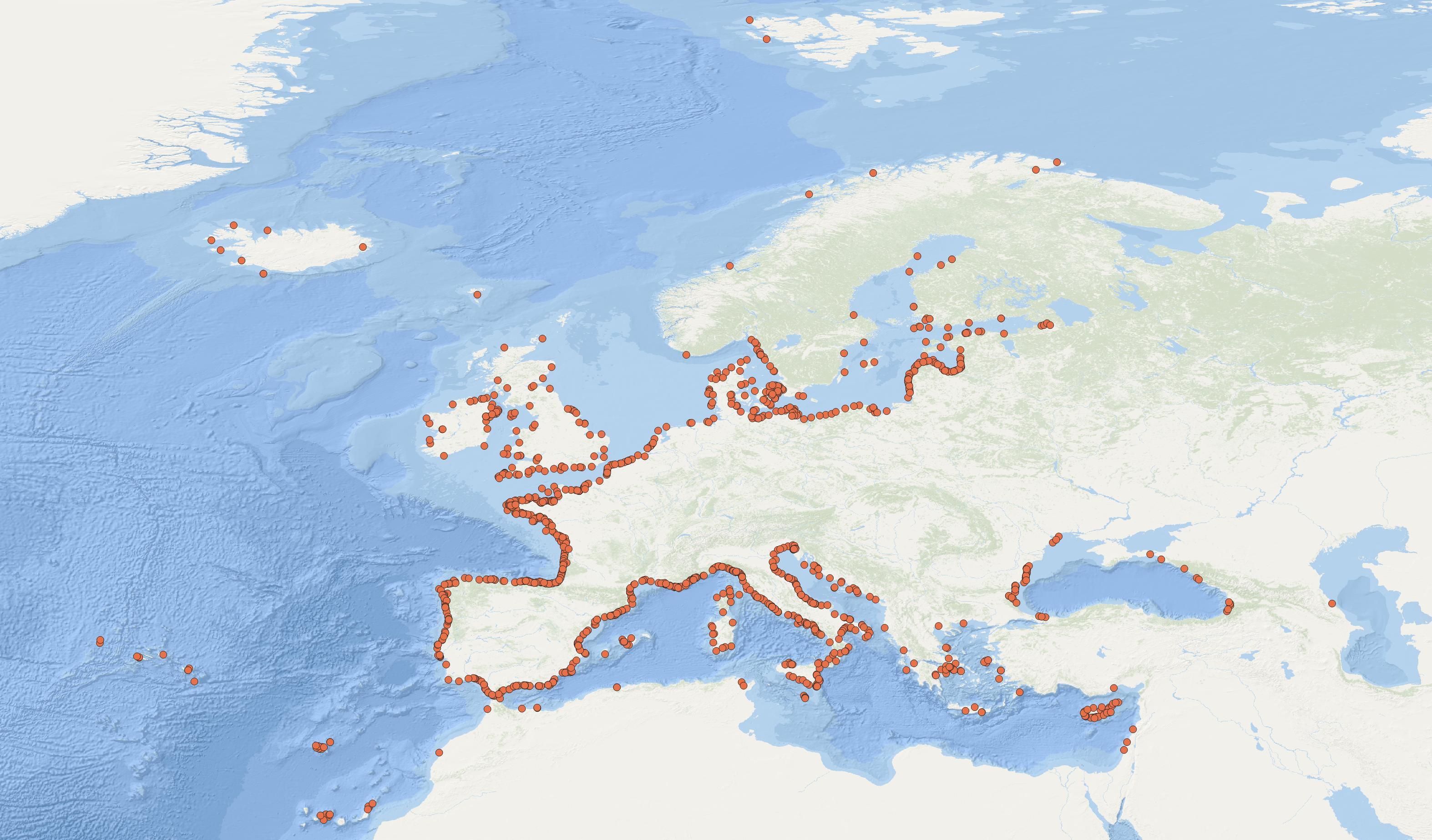
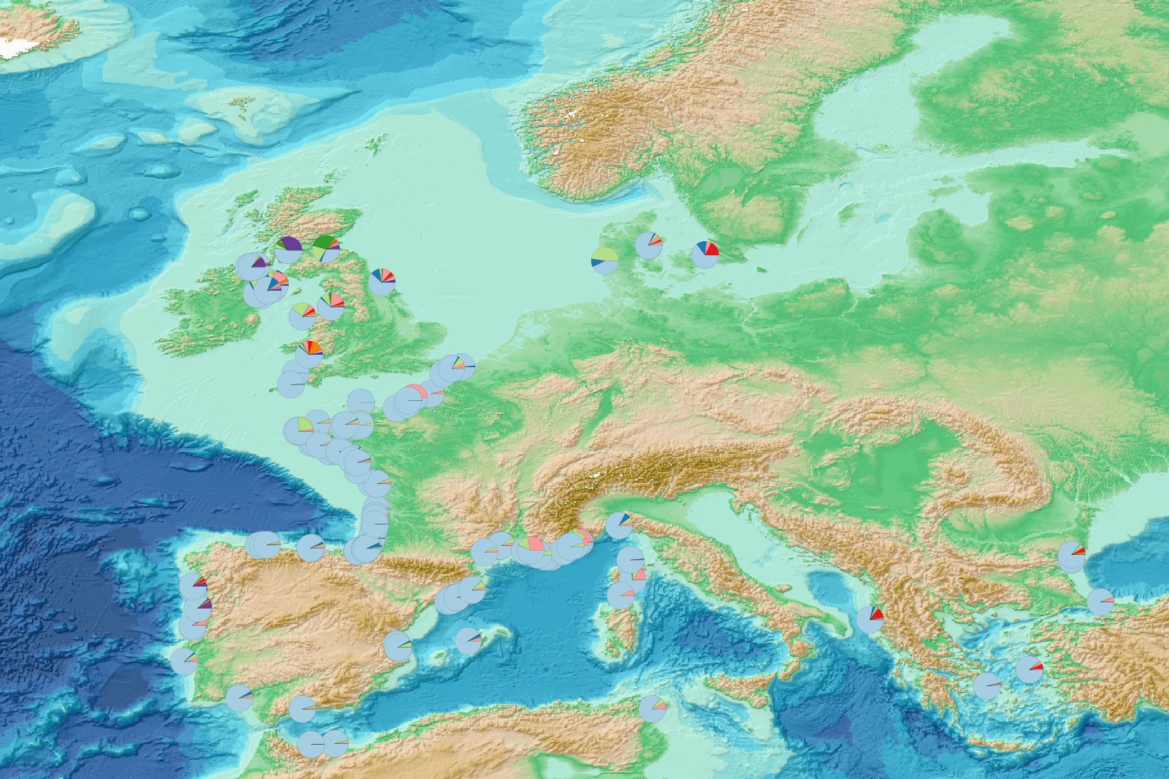
This product displays for Nickel, positions with percentages of all available data values per group of animals that are present in EMODnet regional contaminants aggregated datasets, v2022. The product displays positions for all available years.

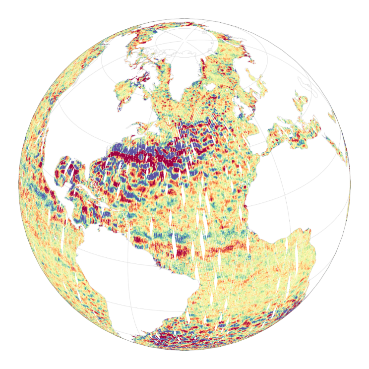
The Level-2 Ka-band Radar Interferometer (KaRIn) low rate (LR, ocean) sea surface height (SSH) data product from the Surface Water and Ocean Topography (SWOT) mission, also referenced by the short name L2_LR_SSH, provides ocean topography measurements from the low rate ocean data stream of the KaRIn instrument, spanning 60 km on either side of the nadir altimeter with a nadir gap. The L2_LR_SSH product is available continuously and globally, although different versions of the product may be produced at different latencies and/or through different reprocessing with refined input data. Note that L2_LR_SSH does not include SSH data from the SWOT nadir altimeter. The SWOT L2_LR_SSH product is organized in four files, the L2_LR_SSH ['Expert'] is described in this metadata sheet. The 3 other file types (['Basic'], ['WindWave'], ['Unsmoothed']) are described by 3 different metadata sheets that can be accessed via the links below. The ['Expert'] file is intended for expert users who are interested in the details of how the KaRIn measurements were derived and who may use detailed information for their own custom processing. The ['Basic'] file is intended for users who are interested in SSH measurements and who will use the KaRIn measurements as provided. The ['WindWave'] file is intended for users interested in wind and wave information. The ['Unsmoothed'] file, also intended for expert users, is provided on a finer 'native' grid of 250-m (with minimal smoothing applied), and has a significantly larger data volume than the other files. The ['Expert'] L2_LR_SSH includes copies of all variables in the Basic and WindWave files (sea surface height (SSH), sea surface height anomaly (SSHA), data quality flags, geophysical reference fields, height correction information, significant wave height (SWH), normalized radar cross section (NRCS or backscatter cross section or sigma0), wind speed derived from sigma0 and SWH, wind and wave model information, quality flags on a 2 km geographically fixed grid), plus more detailed information on the KaRIn instrument and environmental corrections, radiometer data, and geophysical models on a 2 km geographically fixed grid. August 2024: V2.0 L2_LR_SSH version 2.0 (version C) products declared as validated by the SWOT project. March 2024: V2.0 Production and distribution of the pre-validated L2_LR_SSH version 2.0 (or version C) products: - PIC0 for forward-processed version C products: November 23, 2023 to present, - PGC0 for reprocessed version C products: - March 30 to July 10, 2023 (phase CalVal) and from July 26,2023 to January 25, 2024 (phase Science) November 2023: V1.0 The beta pre-validated L2_LR_SSH version 1.0 product (summer 2023 reprocessing release) is available only for the 1-day CalVal orbit phase, from March 29 to July 10, 2023, and the 21-day Science orbit phase from September 7 to November 21, 2023.

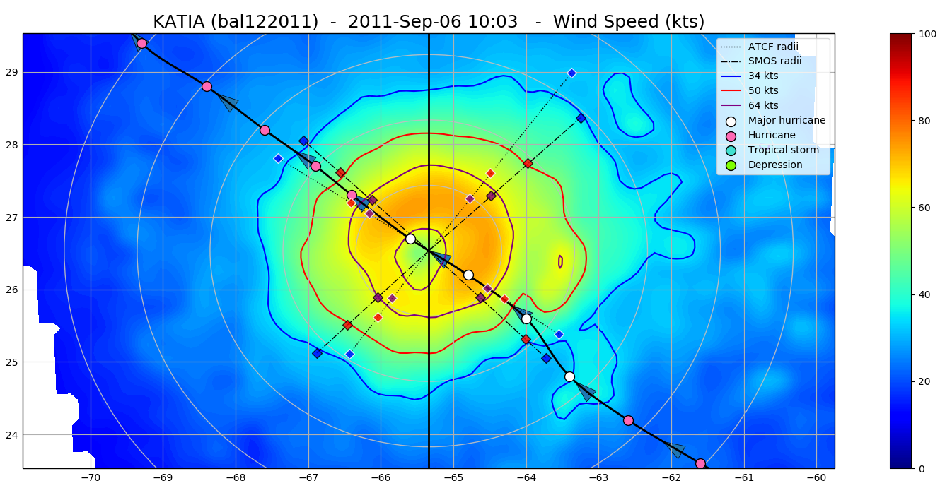
The SMOS WRF product is available in Near Real Time to support tropical cyclones (TC) forecasts. It is generated within 4 to 6 hours from sensing from the SMOS L2 swath wind speed products (SMOS L2WS NRT), in the so-called "Fix (F-deck)" format compatible with the US Navy's ATCF (Automated Tropical Cyclone Forecasting) System. The SMOS WRF "fixes" to the best-track forecasts contain : the SMOS 10-min maximum-sustained winds (in knots) and wind radii (in nautical miles) for the 34 kt (17 m/s), 50 kt (25 m/s) and 64 kt (33 m/s) winds per geographical storm quadrants, and for each SMOS pass intercepting a TC in all the active ocean basins. See the complete description the "SMOS Wind Data Service Product Description Document" ( http://www.smosstorm.org/Document-tools/SMOS-Wind-Data-Service-Documentation ).

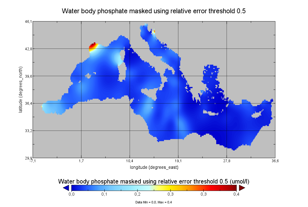
Moving 6-year analysis of Water body phosphate in the Mediterranean Sea for each season: - winter: January-March, - spring: April-June, - summer: July-September, - autumn: October-December. Every year of the time dimension corresponds to the 6-year centered average of the season. 6-years periods span from 1970-1975 until 2017-2022. Data Sources: observational data from SeaDataNet/EMODNet Chemistry Data Network. Units: umol/l. Description of DIVA analysis: The computation was done with the DIVAnd (Data-Interpolating Variational Analysis in n dimensions), version 2.7.9, using GEBCO 30sec topography for the spatial connectivity of water masses. The horizontal resolution of the produced DIVAnd maps grids is dx=dy=0.125 degrees (around 13.5km and 10.9km accordingly). The vertical resolution is 25 depth levels: [0.,5.,10.,20.,30.,50.,75.,100.,125.,150.,200.,250.,300.,400.,500.,600.,700.,800.,900.,1000.,1100.,1200.,1300.,1400.,1500.]. The horizontal correlation length is 200km. The vertical correlation length (in meters) was set twices the vertical resolution: [10.,10.,20.,20.,40.,50.,50.,50.,50.,100.,100.,100.,200.,200.,200.,200.,200.,200.,200.,200.,200.,200.,200.,200.,200.]. Duplicates check was performed using the following criteria for space and time: dlon=0.001deg., dlat=0.001deg., ddepth=1m, dtime=1hour, dvalue=0.1. The error variance (epsilon2) was set equal to 1 for profiles and 10 for time series to reduce the influence of close data near the coasts. An anamorphosis transformation was applied to the data (function DIVAnd.Anam.loglin) to avoid unrealistic negative values: threshold value=200. A background analysis field was used for all years (1970-2022) with correlation length equal to 600km and error variance (epsilon2) equal to 20. Quality control of the observations was applied using the interpolated field (QCMETHOD=3). Residuals (differences between the observations and the analysis (interpolated linearly to the location of the observations) were calculated. Observations with residuals outside the minimum and maximum values of the 99% quantile were discarded from the analysis. Originators of Italian data sets-List of contributors: - Brunetti Fabio (OGS) - Cardin Vanessa, Bensi Manuel doi:10.6092/36728450-4296-4e6a-967d-d5b6da55f306 - Cardin Vanessa, Bensi Manuel, Ursella Laura, Siena Giuseppe doi:10.6092/f8e6d18e-f877-4aa5-a983-a03b06ccb987 - Cataletto Bruno (OGS) - Cinzia Comici Cinzia (OGS) - Civitarese Giuseppe (OGS) - DeVittor Cinzia (OGS) - Giani Michele (OGS) - Kovacevic Vedrana (OGS) - Mosetti Renzo (OGS) - Solidoro C.,Beran A.,Cataletto B.,Celussi M.,Cibic T.,Comici C.,Del Negro P.,De Vittor C.,Minocci M.,Monti M.,Fabbro C.,Falconi C.,Franzo A.,Libralato S.,Lipizer M.,Negussanti J.S.,Russel H.,Valli G., doi:10.6092/e5518899-b914-43b0-8139-023718aa63f5 - Celio Massimo (ARPA FVG) - Malaguti Antonella (ENEA) - Fonda Umani Serena (UNITS) - Bignami Francesco (ISAC/CNR) - Boldrini Alfredo (ISMAR/CNR) - Marini Mauro (ISMAR/CNR) - Miserocchi Stefano (ISMAR/CNR) - Zaccone Renata (IAMC/CNR) - Lavezza, R., Dubroca, L. F. C., Ludicone, D., Kress, N., Herut, B., Civitarese, G., Cruzado, A., Lefèvre, D.,Souvermezoglou, E., Yilmaz, A., Tugrul, S., and Ribera d'Alcala, M.: Compilation of quality controlled nutrient profiles from the Mediterranean Sea, doi:10.1594/PANGAEA.771907, 2011.

'''DEFINITION''' The OMI_EXTREME_SST_MEDSEA_sst_mean_and_anomaly_obs indicator is based on the computation of the 99th and the 1st percentiles from in situ data (observations). It is computed for the variable sea surface temperature measured by in situ buoys at depths between 0 and 5 meters. The use of percentiles instead of annual maximum and minimum values, makes this extremes study less affected by individual data measurement errors. The percentiles are temporally averaged, and the spatial evolution is displayed, jointly with the anomaly in the target year. This study of extreme variability was first applied to sea level variable (Pérez Gómez et al 2016) and then extended to other essential variables, sea surface temperature and significant wave height (Pérez Gómez et al 2018). '''CONTEXT''' Sea surface temperature (SST) is one of the essential ocean variables affected by climate change (mean SST trends, SST spatial and interannual variability, and extreme events). In Europe, several studies show warming trends in mean SST for the last years (von Schuckmann et al., 2016; IPCC, 2021, 2022). An exception seems to be the North Atlantic, where, in contrast, anomalous cold conditions have been observed since 2014 (Mulet et al., 2018; Dubois et al. 2018; IPCC 2021, 2022). Extremes may have a stronger direct influence in population dynamics and biodiversity. According to Alexander et al. 2018 the observed warming trend will continue during the 21st Century and this can result in exceptionally large warm extremes. Monitoring the evolution of sea surface temperature extremes is, therefore, crucial. The Mediterranean Sea has showed a constant increase of the SST in the last three decades across the whole basin with more frequent and severe heat waves (Juza et al., 2022). Deep analyses of the variations have displayed a non-uniform rate in space, being the warming trend more evident in the eastern Mediterranean Sea with respect to the western side. This variation rate is also changing in time over the three decades with differences between the seasons (e.g. Pastor et al. 2018; Pisano et al. 2020), being higher in Spring and Summer, which would affect the extreme values. '''COPERNICUS MARINE SERVICE KEY FINDINGS''' The mean 99th percentiles showed in the area present values from 25ºC in Ionian Sea and 26º in the Alboran sea and Gulf of Lion to 27ºC in the East of Iberian Peninsula. The standard deviation ranges from 0.6ºC to 1.2ºC in the Western Mediterranean and is around 2.2ºC in the Ionian Sea. Results for this year show a slight negative anomaly in the Ionian Sea (-1ºC) inside the standard deviation and a clear positive anomaly in the Western Mediterranean Sea reaching +2.2ºC, almost two times the standard deviation in the area. '''DOI (product):''' https://doi.org/10.48670/moi-00267

This visualization product displays marine macro-litter (> 2.5cm) material categories percentage per beach per year from non-MSFD monitoring surveys, research & cleaning operations. EMODnet Chemistry included the collection of marine litter in its 3rd phase. Since the beginning of 2018, data of beach litter have been gathered and processed in the EMODnet Chemistry Marine Litter Database (MLDB). The harmonization of all the data has been the most challenging task considering the heterogeneity of the data sources, sampling protocols and reference lists used on a European scale. Preliminary processing were necessary to harmonize all the data: - Exclusion of OSPAR 1000 protocol: in order to follow the approach of OSPAR that it is not including these data anymore in the monitoring; - Selection of surveys from non-MSFD monitoring, cleaning and research operations; - Exclusion of beaches without coordinates; - Exclusion of surveys without associated length; - Some litter types like organic litter, small fragments (paraffin and wax; items > 2.5cm) and pollutants have been removed. The list of selected items is attached to this metadata. This list was created using EU Marine Beach Litter Baselines and EU Threshold Value for Macro Litter on Coastlines from JRC (these two documents are attached to this metadata); - Exclusion of the "feaces" category: it concerns more exactly the items of dog excrements in bags of the OSPAR (item code: 121) and ITA (item code: IT59) reference lists; - Normalization of survey lengths to 100m & 1 survey / year: in some case, the survey length was not 100m, so in order to be able to compare the abundance of litter from different beaches a normalization is applied using this formula: Number of items (normalized by 100 m) = Number of litter per items x (100 / survey length) Then, this normalized number of items is summed to obtain the total normalized number of litter for each survey. To calculate percentages for each material category, formula applied is: Material (%) = (∑number of items (normalized at 100 m) of each material category)*100 / (∑number of items (normalized at 100 m) of all categories) The material categories differ between reference lists (OSPAR, TSG_ML, UNEP, UNEP_MARLIN). In order to apply a common procedure for all the surveys, the material categories have been harmonized. More information is available in the attached documents. Warning: the absence of data on the map doesn't necessarily mean that they don't exist, but that no information has been entered in the Marine Litter Database for this area.