 Catalogue PIGMA
oceans
Type of resources
Available actions
Topics
Keywords
Contact for the resource
Provided by
Years
Formats
Representation types
Update frequencies
status
Scale
Resolution
-

'''Short description:''' Le modèle biogéochimique ECO-MARS3D sur la façade Manche Atlantique (PREVIMER_B1-ECOMARS3D-MANGA4000) est un modèle 3D de résolution spatiale 4km qui fournit les concentrations de nutriments et de plancton toutes les heures sur 30 niveaux (fenêtre de prévision à 4 jours). '''Paramètres calculés :''' Les paramètres calculés sont les suivants : * SAL : sea_water_salinity * TEMP : sea_water_temperature * suspended_inorganic_particulate_matter : mass_concentration_of_suspended_matter_in_sea_water * nanopicoplankton_nitrogen : mole_concentration_of_nanoplankton_expressed_as_nitrogen_in_sea_water * diatom_nitrogen : mole_concentration_of_diatoms_expressed_as_nitrogen_in_sea_water * dinoflagellate_nitrogen : mole_concentration_of_dinoflagellates_expressed_as_nitrogen_in_sea_water * microzooplankton_nitrogen : mole_concentration_of_microzooplankton_expressed_as_nitrogen_in_sea_water * mesozooplankton_nitrogen : mole_concentration_of_mesozooplankton_expressed_as_nitrogen_in_sea_water * colonial_phaeocystis_nitrogen : mole_concentration_of_colonial_phaeocystis_expressed_as_nitrogen_in_sea_water * phaeocystis_mucus : concentration_of_phaeocystis_mucus_expressed_as_mass_in_sea_water * ammonium : mole_concentration_of_ammonium_in_sea_water * nitrate : mole_concentration_of_nitrate_in_sea_water * dissolved_silicate : mole_concentration_of_silicate_in_sea_water * dissolved_phosphate : mole_concentration_of_phosphate_in_sea_water * dissolved_oxygen : dissolved_oxygen_in_water_column * cumulative_nanoflagellate_carbon_production : cumulative_nanoflagellate_production_expressed_as_carbon_in_sea_water * cumulative_diatom_carbon_production : cumulative_diatom_production_expressed_as_carbon_in_sea_water * cumulative_dinoflagellate_carbon_production : cumulative_dinoflagellate_production_expressed_as_carbon_in_sea_water * cumulative_phaeocystis_carbon_production : cumulative_phaeocystis_production_expressed_as_carbon_in_sea_water * organic_nitrogen_benth : mole_concentration_of_organic_detritus_expressed_as_nitrogen_in_benthos Les paramètres diagnostiques calculés sont les suivants : * XE : sea_surface_height_above_geoid * maximum_de_diat : maximum_diatom_mass_concentration_in_sea_water * maximum_de_dino : maximum_dinoflagellate_mass_concentration_in_sea_water * maximum_de_nano : maximum_nanoflagellate_mass_concentration_in_sea_water * grad_vert_salinite : maximum_vertical_gradient_of_sea_water_salinity * grad_vert_temp : maximum_vertical_gradient_of_sea_water_temperature * extinction_lumineuse : light_extinction_in_sea_water * prod_diat : cumulated_production_of_diatoms_in_sea_water_column_expressed_in_carbon * prod_dino : cumulated_production_of_dinoflagellates_in_sea_water_column_expressed_in_carbon * prod_nano : cumulated_production_of_nanoflagellates_in_sea_water_column_expressed_in_carbon * chlorophylle_a : chlorophyll_mass_concentration_in_sea_water * prod_cumul_chloro : cumulated_total_production_in_sea_water_column_expressed_in_carbon * maximum_de_phaeocystis : maximum_phaeocystis_mass_concentration_in_sea_water * prod_phaeocystis : cumulated_production_of_phaeocystis_in_sea_water_column_expressed_in_carbon * oxygen_saturation : oxygen_saturation * ammoniumGIRON_tracer_sign: mole_concentration_of_ammonium_in_sea_waterGIRON_tracer_sign * ammoniumGIRON_tracer_age: mole_concentration_of_ammonium_in_sea_waterGIRON_tracer_age * nitrateGIRON_tracer_sign: mole_concentration_of_nitrate_in_sea_waterGIRON_tracer_sign * nitrateGIRON_tracer_age: mole_concentration_of_nitrate_in_sea_waterGIRON_tracer_age * nanopicoplankton_nitrogenGIRON_tracer_sign: mole_concentration_of_nanoplankton_expressed_as_nitrogen_in_sea_waterGIRON_tracer_sign * nanopicoplankton_nitrogenGIRON_tracer_age: mole_concentration_of_nanoplankton_expressed_as_nitrogen_in_sea_waterGIRON_tracer_age * diatom_nitrogenGIRON_tracer_sign: mole_concentration_of_diatoms_expressed_as_nitrogen_in_sea_waterGIRON_tracer_sign * diatom_nitrogenGIRON_tracer_age: mole_concentration_of_diatoms_expressed_as_nitrogen_in_sea_waterGIRON_tracer_age * dinoflagellate_nitrogenGIRON_tracer_sign: mole_concentration_of_dinoflagellates_expressed_as_nitrogen_in_sea_waterGIRON_tracer_sign * dinoflagellate_nitrogenGIRON_tracer_age: mole_concentration_of_dinoflagellates_expressed_as_nitrogen_in_sea_waterGIRON_tracer_age * microzooplankton_nitrogenGIRON_tracer_sign: mole_concentration_of_microzooplankton_expressed_as_nitrogen_in_sea_waterGIRON_tracer_sign * microzooplankton_nitrogenGIRON_tracer_age: mole_concentration_of_microzooplankton_expressed_as_nitrogen_in_sea_waterGIRON_tracer_age * mesozooplankton_nitrogenGIRON_tracer_sign: mole_concentration_of_mesozooplankton_expressed_as_nitrogen_in_sea_waterGIRON_tracer_sign * mesozooplankton_nitrogenGIRON_tracer_age: mole_concentration_of_mesozooplankton_expressed_as_nitrogen_in_sea_waterGIRON_tracer_age * detrital_nitrogenGIRON_tracer_sign: mole_concentration_of_organic_detritus_expressed_as_nitrogen_in_sea_waterGIRON_tracer_sign * detrital_nitrogenGIRON_tracer_age: mole_concentration_of_organic_detritus_expressed_as_nitrogen_in_sea_waterGIRON_tracer_age * colonial_phaeocystis_nitrogenGIRON_tracer_sign: mole_concentration_of_colonial_phaeocystis_expressed_as_nitrogen_in_sea_waterGIRON_tracer_sign * colonial_phaeocystis_nitrogenGIRON_tracer_age: mole_concentration_of_colonial_phaeocystis_expressed_as_nitrogen_in_sea_waterGIRON_tracer_age * phaeocystis_cells_nitrogenGIRON_tracer_sign: mole_concentration_of_phaeocystis_cells_expressed_as_nitrogen_in_sea_waterGIRON_tracer_sign * phaeocystis_cells_nitrogenGIRON_tracer_age: mole_concentration_of_phaeocystis_cells_expressed_as_nitrogen_in_sea_waterGIRON_tracer_age * organic_nitrogen_benthGIRON_tracer_sign: mole_concentration_of_organic_detritus_expressed_as_nitrogen_in_benthosGIRON_tracer_sign * organic_nitrogen_benthGIRON_tracer_age: mole_concentration_of_organic_detritus_expressed_as_nitrogen_in_benthosGIRON_tracer_age * phytoplankton_sign_N_GIRON: nitrogen_fraction_in_phytoplankton_from_source_GIRON * phytoplankton_age_N_GIRON: age_of_nitrogen_fraction_in_phytoplankton_from_source_GIRON * ammoniumLOIRE_tracer_sign: mole_concentration_of_ammonium_in_sea_waterLOIRE_tracer_sign * ammoniumLOIRE_tracer_age: mole_concentration_of_ammonium_in_sea_waterLOIRE_tracer_age * nitrateLOIRE_tracer_sign: mole_concentration_of_nitrate_in_sea_waterLOIRE_tracer_sign * nitrateLOIRE_tracer_age: mole_concentration_of_nitrate_in_sea_waterLOIRE_tracer_age * nanopicoplankton_nitrogenLOIRE_tracer_sign: mole_concentration_of_nanoplankton_expressed_as_nitrogen_in_sea_waterLOIRE_tracer_sign * nanopicoplankton_nitrogenLOIRE_tracer_age: mole_concentration_of_nanoplankton_expressed_as_nitrogen_in_sea_waterLOIRE_tracer_age * diatom_nitrogenLOIRE_tracer_sign: mole_concentration_of_diatoms_expressed_as_nitrogen_in_sea_waterLOIRE_tracer_sign * diatom_nitrogenLOIRE_tracer_age: mole_concentration_of_diatoms_expressed_as_nitrogen_in_sea_waterLOIRE_tracer_age * dinoflagellate_nitrogenLOIRE_tracer_sign: mole_concentration_of_dinoflagellates_expressed_as_nitrogen_in_sea_waterLOIRE_tracer_sign * dinoflagellate_nitrogenLOIRE_tracer_age: mole_concentration_of_dinoflagellates_expressed_as_nitrogen_in_sea_waterLOIRE_tracer_age * microzooplankton_nitrogenLOIRE_tracer_sign: mole_concentration_of_microzooplankton_expressed_as_nitrogen_in_sea_waterLOIRE_tracer_sign * microzooplankton_nitrogenLOIRE_tracer_age: mole_concentration_of_microzooplankton_expressed_as_nitrogen_in_sea_waterLOIRE_tracer_age * mesozooplankton_nitrogenLOIRE_tracer_sign: mole_concentration_of_mesozooplankton_expressed_as_nitrogen_in_sea_waterLOIRE_tracer_sign * mesozooplankton_nitrogenLOIRE_tracer_age: mole_concentration_of_mesozooplankton_expressed_as_nitrogen_in_sea_waterLOIRE_tracer_age * detrital_nitrogenLOIRE_tracer_sign: mole_concentration_of_organic_detritus_expressed_as_nitrogen_in_sea_waterLOIRE_tracer_sign * detrital_nitrogenLOIRE_tracer_age: mole_concentration_of_organic_detritus_expressed_as_nitrogen_in_sea_waterLOIRE_tracer_age * colonial_phaeocystis_nitrogenLOIRE_tracer_sign: mole_concentration_of_colonial_phaeocystis_expressed_as_nitrogen_in_sea_waterLOIRE_tracer_sign * colonial_phaeocystis_nitrogenLOIRE_tracer_age: mole_concentration_of_colonial_phaeocystis_expressed_as_nitrogen_in_sea_waterLOIRE_tracer_age * phaeocystis_cells_nitrogenLOIRE_tracer_sign: mole_concentration_of_phaeocystis_cells_expressed_as_nitrogen_in_sea_waterLOIRE_tracer_sign * phaeocystis_cells_nitrogenLOIRE_tracer_age: mole_concentration_of_phaeocystis_cells_expressed_as_nitrogen_in_sea_waterLOIRE_tracer_age * organic_nitrogen_benthLOIRE_tracer_sign: mole_concentration_of_organic_detritus_expressed_as_nitrogen_in_benthosLOIRE_tracer_sign * organic_nitrogen_benthLOIRE_tracer_age: mole_concentration_of_organic_detritus_expressed_as_nitrogen_in_benthosLOIRE_tracer_age * phytoplankton_sign_N_LOIRE: nitrogen_fraction_in_phytoplankton_from_source_LOIRE * phytoplankton_age_N_LOIRE: age_of_nitrogen_fraction_in_phytoplankton_from_source_LOIRE * ammoniumSEINE_tracer_sign: mole_concentration_of_ammonium_in_sea_waterSEINE_tracer_sign * ammoniumSEINE_tracer_age: mole_concentration_of_ammonium_in_sea_waterSEINE_tracer_age * nitrateSEINE_tracer_sign: mole_concentration_of_nitrate_in_sea_waterSEINE_tracer_sign * nitrateSEINE_tracer_age: mole_concentration_of_nitrate_in_sea_waterSEINE_tracer_age * nanopicoplankton_nitrogenSEINE_tracer_sign: mole_concentration_of_nanoplankton_expressed_as_nitrogen_in_sea_waterSEINE_tracer_sign * nanopicoplankton_nitrogenSEINE_tracer_age: mole_concentration_of_nanoplankton_expressed_as_nitrogen_in_sea_waterSEINE_tracer_age * diatom_nitrogenSEINE_tracer_sign: mole_concentration_of_diatoms_expressed_as_nitrogen_in_sea_waterSEINE_tracer_sign * diatom_nitrogenSEINE_tracer_age: mole_concentration_of_diatoms_expressed_as_nitrogen_in_sea_waterSEINE_tracer_age * dinoflagellate_nitrogenSEINE_tracer_sign: mole_concentration_of_dinoflagellates_expressed_as_nitrogen_in_sea_waterSEINE_tracer_sign * dinoflagellate_nitrogenSEINE_tracer_age: mole_concentration_of_dinoflagellates_expressed_as_nitrogen_in_sea_waterSEINE_tracer_age * microzooplankton_nitrogenSEINE_tracer_sign: mole_concentration_of_microzooplankton_expressed_as_nitrogen_in_sea_waterSEINE_tracer_sign * microzooplankton_nitrogenSEINE_tracer_age: mole_concentration_of_microzooplankton_expressed_as_nitrogen_in_sea_waterSEINE_tracer_age * mesozooplankton_nitrogenSEINE_tracer_sign: mole_concentration_of_mesozooplankton_expressed_as_nitrogen_in_sea_waterSEINE_tracer_sign * mesozooplankton_nitrogenSEINE_tracer_age: mole_concentration_of_mesozooplankton_expressed_as_nitrogen_in_sea_waterSEINE_tracer_age * detrital_nitrogenSEINE_tracer_sign: mole_concentration_of_organic_detritus_expressed_as_nitrogen_in_sea_waterSEINE_tracer_sign * detrital_nitrogenSEINE_tracer_age: mole_concentration_of_organic_detritus_expressed_as_nitrogen_in_sea_waterSEINE_tracer_age * colonial_phaeocystis_nitrogenSEINE_tracer_sign: mole_concentration_of_colonial_phaeocystis_expressed_as_nitrogen_in_sea_waterSEINE_tracer_sign * colonial_phaeocystis_nitrogenSEINE_tracer_age: mole_concentration_of_colonial_phaeocystis_expressed_as_nitrogen_in_sea_waterSEINE_tracer_age * phaeocystis_cells_nitrogenSEINE_tracer_sign: mole_concentration_of_phaeocystis_cells_expressed_as_nitrogen_in_sea_waterSEINE_tracer_sign * phaeocystis_cells_nitrogenSEINE_tracer_age: mole_concentration_of_phaeocystis_cells_expressed_as_nitrogen_in_sea_waterSEINE_tracer_age * organic_nitrogen_benthSEINE_tracer_sign: mole_concentration_of_organic_detritus_expressed_as_nitrogen_in_benthosSEINE_tracer_sign * organic_nitrogen_benthSEINE_tracer_age: mole_concentration_of_organic_detritus_expressed_as_nitrogen_in_benthosSEINE_tracer_age * phytoplankton_sign_N_SEINE: nitrogen_fraction_in_phytoplankton_from_source_SEINE * phytoplankton_age_N_SEINE: age_of_nitrogen_fraction_in_phytoplankton_from_source_SEINE
-

Google Earth Engine combines a multi-petabyte catalog of satellite imagery and geospatial datasets with planetary-scale analysis capabilities. Scientists, researchers, and developers use Earth Engine to detect changes, map trends, and quantify differences on the Earth's surface. Earth Engine is now available for commercial use, and remains free for academic and research use.
-
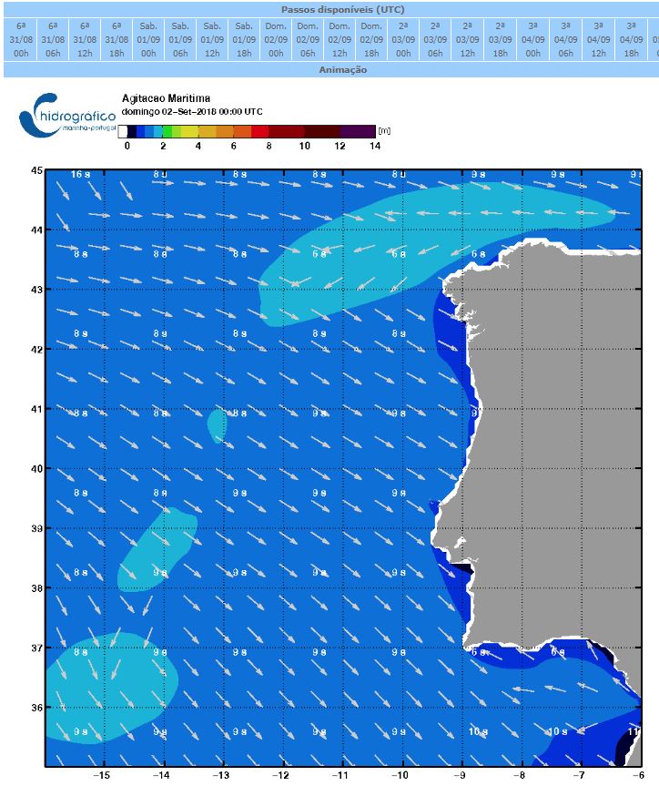
he Hydrographic Institute of Portugal collects and disseminates to a wide user community useful hydrographic/oceanographic information.
-

rgbif is an R package from rOpenSci that allows searching and retrieving data from GBIF. rgbif wraps R code around the GBIF API to allow you to talk to GBIF from R and access metadata, species names, and occurrences. rgbif allows you to easily: - get data for single occurrences - retrieve multiple occurences - search for taxon names - generate maps of occurences
-
Combined product of Water body phosphate based on DIVA 4D 10-year analysis on five regions : Northeast Atlantic Ocean, North Sea, Baltic Sea, Black Sea, Mediterranean Sea. The boundaries and overlapping zones between these five regions were filtered to avoid any unrealistic spatial discontinuities. This combined water body phosphate product is masked using the relative error threshold 0.5. Units: umol/l
-

'''Short description:''' For the NWS/IBI Ocean- Sea Surface Temperature L3 Observations . This product provides daily foundation sea surface temperature from multiple satellite sources. The data are intercalibrated. This product consists in a fusion of sea surface temperature observations from multiple satellite sensors, daily, over a 0.05° resolution grid. It includes observations by polar orbiting from the ESA CCI / C3S archive . The L3S SST data are produced selecting only the highest quality input data from input L2P/L3P images within a strict temporal window (local nightime), to avoid diurnal cycle and cloud contamination. The observations of each sensor are intercalibrated prior to merging using a bias correction based on a multi-sensor median reference correcting the large-scale cross-sensor biases. '''DOI (product) :''' https://doi.org/10.48670/moi-00311
-
Seabed Habitats was one of seven themes of the European Marine Observation and Data Network (EMODnet) initiative, funded by the European Maritime and Fisheries Fund. Since its inception in 2009, EMODnet Seabed Habitats developed, improved and gradually increased the coverage of a broad-scale seabed habitat map for Europe's seabed, also known as EUSeaMap. In addition, EMODnet Seabed Habitats continued the work started by MESH and MESH Atlantic projects in collating and making available seabed habitat maps from surveys, through the EMODnet Seabed Habitats map viewer. In it's third Phase (2017-2019), EMODnet Seabed Habitats collated and provided habitat point data and the outputs of habitat distribution modelling, and the third phase has now been extended to 2021. The extended third phase of the project will: - Continue to grow Europe's only comprehensive library of habitat maps from surveys and collection of survey sample points - Create new composite data products to add to those for the Essential Ocean Variable habitats and OSPAR threatened and/or declining habitats - Update the EMODnet broad-scale seabed habitat map for Europe (EUSeaMap) using the next seabed substrate update from EMODnet Geology - Update web content with extra resources for habitat mapping, including a catalogue highlighting all the most useful data products
-
-
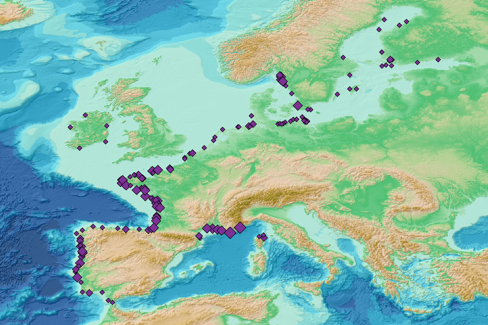
This visualization product displays the total abundance of marine macro-litter (> 2.5cm) per beach per year from Marine Strategy Framework Directive (MSFD) monitoring surveys. EMODnet Chemistry included the collection of marine litter in its 3rd phase. Since the beginning of 2018, data of beach litter have been gathered and processed in the EMODnet Chemistry Marine Litter Database (MLDB). The harmonization of all the data has been the most challenging task considering the heterogeneity of the data sources, sampling protocols and reference lists used on a European scale. Preliminary processings were necessary to harmonize all the data: - Exclusion of OSPAR 1000 protocol: in order to follow the approach of OSPAR that it is not including these data anymore in the monitoring; - Selection of MSFD surveys only (exclusion of other monitoring, cleaning and research operations); - Exclusion of beaches without coordinates; - Some categories & some litter types like organic litter, small fragments (paraffin and wax; items > 2.5cm) and pollutants have been removed. The list of selected items is attached to this metadata. This list was created using EU Marine Beach Litter Baselines, the European Threshold Value for Macro Litter on Coastlines and the Joint list of litter categories for marine macro-litter monitoring from JRC (these three documents are attached to this metadata); - Normalization of survey lengths to 100m & 1 survey / year: in some cases, the survey length was not exactly 100m, so in order to be able to compare the abundance of litter from different beaches a normalization is applied using this formula: Number of items (normalized by 100 m) = Number of litter per items x (100 / survey length) Then, this normalized number of items is summed to obtain the total normalized number of litter for each survey. Finally, the median abundance for each beach and year is calculated from these normalized abundances per survey. Sometimes the survey length was null or equal to 0. Assuming that the MSFD protocol has been applied, the length has been set at 100m in these cases. Percentiles 50, 75, 95 & 99 have been calculated taking into account MSFD data for all years. More information is available in the attached documents. Warning: the absence of data on the map does not necessarily mean that it does not exist, but that no information has been entered in the Marine Litter Database for this area.
-
