'''DEFINITION''' Ocean heat content (OHC) is defined here as the deviation from a reference period (1993-2014) and is closely proportional to the average temperature change from z1 = 0 m to z2 = 700 m depth: OHC=∫_(z_1)^(z_2)ρ_0 c_p (T_yr-T_clim )dz [1] with a reference density of = 1030 kgm-3 and a specific heat capacity of cp = 3980 J kg-1 °C-1 (e.g. von Schuckmann et al., 2009). Time series of annual mean values area averaged ocean heat content is provided for the Mediterranean Sea (30°N, 46°N; 6°W, 36°E) and is evaluated for topography deeper than 300m. '''CONTEXT''' Knowing how much and where heat energy is stored and released in the ocean is essential for understanding the contemporary Earth system state, variability and change, as the oceans shape our perspectives for the future. The quality evaluation of MEDSEA_OMI_OHC_area_averaged_anomalies is based on the “multi-product” approach as introduced in the second issue of the Ocean State Report (von Schuckmann et al., 2018), and following the MyOcean’s experience (Masina et al., 2017). Six global products and a regional (Mediterranean Sea) product have been used to build an ensemble mean, and its associated ensemble spread. The reference products are: • The Mediterranean Sea Reanalysis at 1/24 degree horizontal resolution (MEDSEA_MULTIYEAR_PHY_006_004, DOI: https://doi.org/10.25423/CMCC/MEDSEA_MULTIYEAR_PHY_006_004_E3R1, Escudier et al., 2020) • Four global reanalyses at 1/4 degree horizontal resolution (GLOBAL_MULTIYEAR_PHY_ENS_001_031): GLORYS, C-GLORS, ORAS5, FOAM • Two observation based products: CORA (INSITU_GLO_PHY_TS_OA_MY_013_052) and ARMOR3D (MULTIOBS_GLO_PHY_TSUV_3D_MYNRT_015_012). Details on the products are delivered in the PUM and QUID of this OMI. '''CMEMS KEY FINDINGS''' The ensemble mean ocean heat content anomaly time series over the Mediterranean Sea shows a continuous increase in the period 1993-2022 at rate of 1.38±0.08 W/m2 in the upper 700m. After 2005 the rate has clearly increased with respect the previous decade, in agreement with Iona et al. (2018). '''DOI (product):''' https://doi.org/10.48670/moi-00261

'''DEFINITION''' Estimates of Ocean Heat Content (OHC) are obtained from integrated differences of the measured temperature and a climatology along a vertical profile in the ocean (von Schuckmann et al., 2018). The products used include three global reanalyses: GLORYS, C-GLORS, ORAS5 (GLOBAL_MULTIYEAR_PHY_ENS_001_031) and two in situ based reprocessed products: CORA5.2 (INSITU_GLO_PHY_TS_OA_MY_013_052) , ARMOR-3D (MULTIOBS_GLO_PHY_TSUV_3D_MYNRT_015_012). Additionally, the time series based on the method of von Schuckmann and Le Traon (2011) has been added. The regional OHC values are then averaged from 60°S-60°N aiming i) to obtain the mean OHC as expressed in Joules per meter square (J/m2) to monitor the large-scale variability and change. ii) to monitor the amount of energy in the form of heat stored in the ocean (i.e. the change of OHC in time), expressed in Watt per square meter (W/m2). Ocean heat content is one of the six Global Climate Indicators recommended by the World Meterological Organisation for Sustainable Development Goal 13 implementation (WMO, 2017). '''CONTEXT''' Knowing how much and where heat energy is stored and released in the ocean is essential for understanding the contemporary Earth system state, variability and change, as the ocean shapes our perspectives for the future (von Schuckmann et al., 2020). Variations in OHC can induce changes in ocean stratification, currents, sea ice and ice shelfs (IPCC, 2019; 2021); they set time scales and dominate Earth system adjustments to climate variability and change (Hansen et al., 2011); they are a key player in ocean-atmosphere interactions and sea level change (WCRP, 2018) and they can impact marine ecosystems and human livelihoods (IPCC, 2019). '''CMEMS KEY FINDINGS''' Since the year 2005, the upper (0-700m) near-global (60°S-60°N) ocean warms at a rate of 0.6 ± 0.1 W/m2. Note: The key findings will be updated annually in November, in line with OMI evolutions. '''DOI (product):''' https://doi.org/10.48670/moi-00234

The Mytilobs network, carried out by IFREMER (French Research Institute for Exploitation of the Sea), is a national network dedicated to building long-term physiological variations time series of blue mussels (Mytilus edulis), across a large spatial scale. This observation network, initially designed to survey production yields, also provides valuable data to track environmental variations of coastal ecosystems. Mussels exhibit high phenotypic plasticity in response to environmental variations. Collection of data describing phenotypic variations, over an extended period, reveals small-scale climate and habitat variations. With its broad deployment across time and space, the data produced under Mytilobs will be useful for the establishment of a baseline condition when studying the effect of a perturbation affecting an ecosystem’s functioning. Finally, the monitoring of mussel biometric traits and mortality was coupled with high-frequency measurements of salinity, temperature, and sea level, complementing this multi-layer observational framework.

This visualization product displays the marine litter material categories percentage per trawl. EMODnet Chemistry included the collection of marine litter in its 3rd phase. Since the beginning of 2018, data of seafloor litter collected by international fish-trawl surveys have been gathered and processed in the EMODnet Chemistry Marine Litter Database (MLDB). The harmonization of all the data has been the most challenging task considering the heterogeneity of the data sources, sampling protocols (OSPAR and MEDITS protocols) and reference lists used on a European scale. Moreover, within the same protocol, different gear types are deployed during bottom trawl surveys. Unlike other EMODnet seafloor litter products, all trawls surveyed since 2007 are included in this map even if the wingspread and/or the distance are/is unknown. Only surveys with an unknown number of items were excluded from this product. Harmonization of the material categories between ICES and MEDITS lists was performed and the following calculation was applied: Material % = (∑Number of items of each material category*100)/(∑Number of items of all material categories) More information on data processing and calculation are detailed in the attached document. Warning: the absence of data on the map does not necessarily mean that they do not exist, but that no information has been entered in the Marine Litter Database for this area.

The raster corresponds to the predicted Mediterranean bioregions of megabenthic communities.

This visualization product displays nets locations (start positions) where specific protocols have been applied to collate data on microlitter. Mesh size used with these protocols have been indicated with different colors in the map. EMODnet Chemistry included the collection of marine litter in its 3rd phase. Before 2021, there was no coordinated effort at the regional or European scale for micro-litter. Given this situation, EMODnet Chemistry proposed to adopt the data gathering and data management approach as generally applied for marine data, i.e., populating metadata and data in the CDI Data Discovery and Access service using dedicated SeaDataNet data transport formats. EMODnet Chemistry is currently the official EU collector of micro-litter data from Marine Strategy Framework Directive (MSFD) National Monitoring activities (descriptor 10). A series of specific standard vocabularies or standard terms related to micro-litter have been added to SeaDataNet NVS (NERC Vocabulary Server) Common Vocabularies to describe the micro-litter. European micro-litter data are collected by the National Oceanographic Data Centres (NODCs). Micro-litter map products are generated from NODCs data after a test of the aggregated collection including data and data format checks and data harmonization. A filter is applied to represent only micro-litter sampled according to a very specific protocol such as the Volvo Ocean Race (VOR) or Oceaneye. Warning: the absence of data on the map does not necessarily mean that they do not exist, but that no information has been entered in the National Oceanographic Data Centre (NODC) for this area.

This visualization product displays nets locations where research and monitoring protocols have been applied to collate data on microlitter. Mesh size used with these protocols have been indicated with different colors in the map. EMODnet Chemistry included the collection of marine litter in its 3rd phase. Before 2021, there was no coordinated effort at the regional or European scale for micro-litter. Given this situation, EMODnet Chemistry proposed to adopt the data gathering and data management approach as generally applied for marine data, i.e., populating metadata and data in the CDI Data Discovery and Access service using dedicated SeaDataNet data transport formats. EMODnet Chemistry is currently the official EU collector of micro-litter data from Marine Strategy Framework Directive (MSFD) National Monitoring activities (descriptor 10). A series of specific standard vocabularies or standard terms related to micro-litter have been added to SeaDataNet NVS (NERC Vocabulary Server) Common Vocabularies to describe the micro-litter. European micro-litter data are collected by the National Oceanographic Data Centres (NODCs). Micro-litter map products are generated from NODCs data after a test of the aggregated collection including data and data format checks and data harmonization. A filter is applied to represent only micro-litter sampled according to research and monitoring protocols as MSFD monitoring. Warning: the absence of data on the map does not necessarily mean that they do not exist, but that no information has been entered in the National Oceanographic Data Centre (NODC) for this area.

Plankton was sampled with a Continuous Underway Fish Egg Sampler (CUFES, 315µm mesh size) at 4 m below the surface, and a WP2 net (200µm mesh size) from 100m to the surface, or 5 m above the sea floor to the surface when the depth was < 100 m, in the Bay of Biscay. The full images were processed with the ZooCAM software and the embedded Matrox Imaging Library (Colas et a., 2018) which generated regions of interest (ROIs) around each individual object and a set of features measured on the object. The same objects were re-processed to compute features with the scikit-image library http://scikit-image.org. The 1, 286, 590 resulting objects were sorted by a limited number of operators, following a common taxonomic guide, into 93 taxa, using the web application EcoTaxa http://ecotaxa.obs-vlfr.fr. For the purpose of training machine learning classifiers, the images in each class were split into training, validation, and test sets, with proportions 70%, 15% and 15%. The archive contains : taxa.csv.gz Table of the classification of each object in the dataset, with columns : - objid : unique object identifier in EcoTaxa (integer number). - taxon_level1 : taxonomic name corresponding to the level 1 classification - lineage_level1 : taxonomic lineage corresponding to the level 1 classification - taxon_level2 : name of the taxon corresponding to the level 2 classification  - plankton : if the object is a plankton or not (boolean) - set : class of the image corresponding to the taxon (train : training, val : validation, or test) - img_path : local path of the image corresponding to the taxon (of level 1), named according to the object id features_native.csv.gz Table of morphological features computed by ZooCAM. All features are computed on the object only, not the background. All area/length measures are in pixels. All grey levels are in encoded in 8 bits (0=black, 255=white). With columns : - area : object's surface - area_exc : object surface excluding white pixels - area_based_diameter : object's Area Based Diameter: 2 * (object_area/pi)^(1/2) - meangreyobjet : mean image grey level - modegreyobjet : modal object grey level - sigmagrey : object grey level standard deviation - mingrey : minimum object grey level - maxgrey : maximum object grey level - sumgrey : object grey level integrated density: object_mean*object_area - breadth : breadth of the object along the best fitting ellipsoid minor axis - length : breadth of the object along the best fitting ellipsoid majorr axis - elongation : elongation index: object_length/object_breadth - perim : object's perimeter - minferetdiam : minimum object's feret diameter - maxferetdiam : maximum object's feret diameter - meanferetdiam : average object's feret diameter - feretelongation : elongation index: object_maxferetdiam/object_minferetdiam - compactness : Isoperimetric quotient: the ration of the object's area to the area of a circle having the same perimeter - intercept0, intercept45 , intercept90, intercept135 : the number of times that a transition from background to foreground occurs a the angle 0ø, 45ø, 90ø and 135ø for the entire object - convexhullarea : area of the convex hull of the object - convexhullfillratio : ratio object_area/convexhullarea - convexperimeter : perimeter of the convex hull of the object - n_number_of_runs : number of horizontal strings of consecutive foreground pixels in the object - n_chained_pixels : number of chained pixels in the object - n_convex_hull_points : number of summits of the object's convex hull polygon - n_number_of_holes : number of holes (as closed white pixel area) in the object - roughness : measure of small scale variations of amplitude in the object's grey levels - rectangularity : ratio of the object's area over its best bounding rectangle's area - skewness : skewness of the object's grey level distribution - kurtosis : kurtosis of the object's grey level distribution - fractal_box : fractal dimension of the object's perimeter - hist25, hist50, hist75 : grey level value at quantile 0.25, 0.5 and 0.75 of the object's grey levels normalized cumulative histogram - valhist25, valhist50, valhist75 : sum of grey levels at quantile 0.25, 0.5 and 0.75 of the object's grey levels normalized cumulative histogram - nobj25, nobj50, nobj75 : number of objects after thresholding at the object_valhist25, object_valhist50 and object_valhist75 grey level - symetrieh :index of horizontal symmetry - symetriev : index of vertical symmetry - skelarea : area of the object skeleton - thick_r : maximum object's thickness/mean object's thickness - cdist : distance between the mass and the grey level object's centroids features_skimage.csv.gz Table of morphological features recomputed with skimage.measure.regionprops on the ROIs produced by ZooCAM. See http://scikit-image.org/docs/dev/api/skimage.measure.html#skimage.measure.regionprops for documentation. inventory.tsv Tree view of the taxonomy and number of images in each taxon, displayed as text. With columns : - lineage_level1 : taxonomic lineage corresponding to the level 1 classification - taxon_level1 : name of the taxon corresponding to the level 1 classification - n : number of objects in each taxon group map.png Map of the sampling locations, to give an idea of the diversity sampled in this dataset. imgs Directory containing images of each object, named according to the object id objid and sorted in subdirectories according to their taxon.

As part of the marine water quality monitoring of the “Pertuis” and the “baie de l’Aiguillon” (France), commissioned by the OFB and carried out by setec énergie environnement, three monitoring stations were installed. Two of them were set up at the mouths of the Charente and Seudre rivers on February 6 and 27, 2019, respectively, while a third was deployed in the Bay of Aiguillon on March 24, 2021. The dataset presented here concerns the station installed in the Bay of Aiguillon. Measurements are organized into .csv files, with one file per year. Data is collected using a WiMO multiparameter probe, which records the following parameters: •    Temperature (-2 to 35 °C) •    Conductivity (0 to 100 mS/cm) •    Pressure (0 to 30 m) •    Turbidity (0 to 4000 NTU) •    Dissolved Oxygen (0 to 23 mg/L & 0 to 250 %) •    Fluorescence (0 to 500 ppb)  

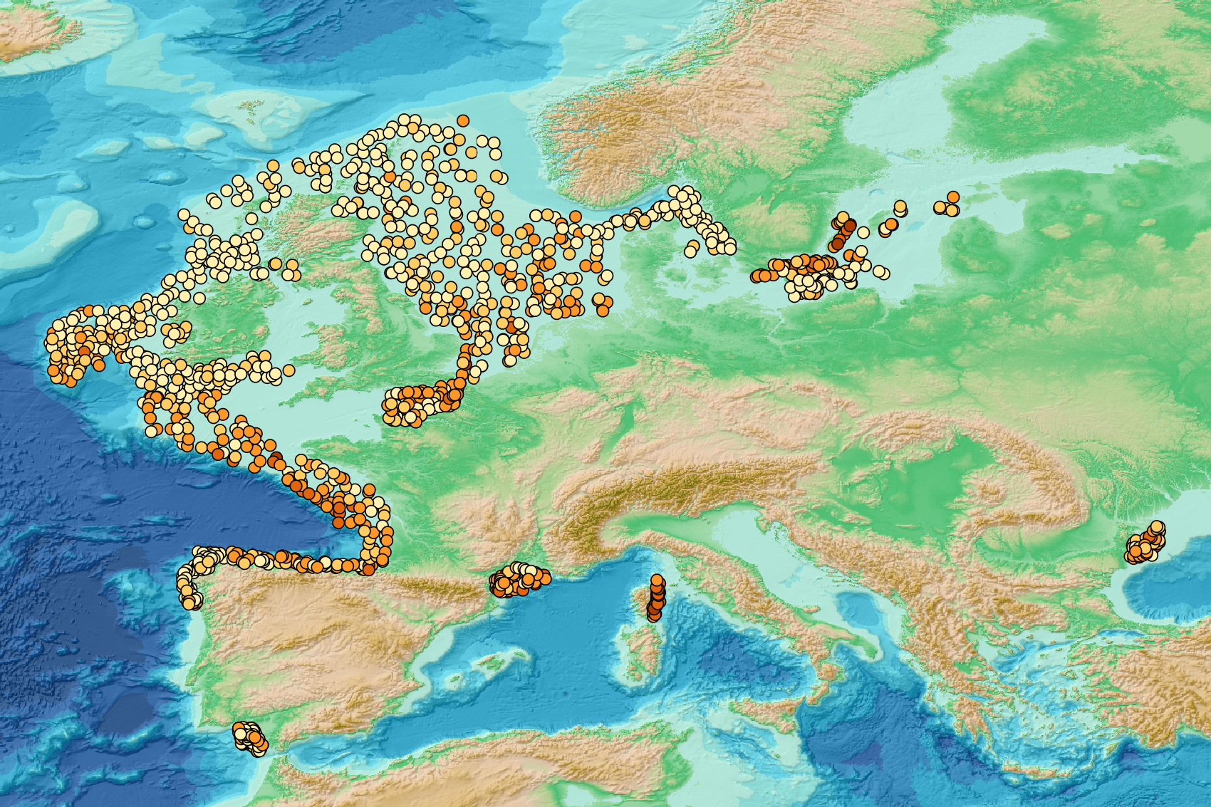
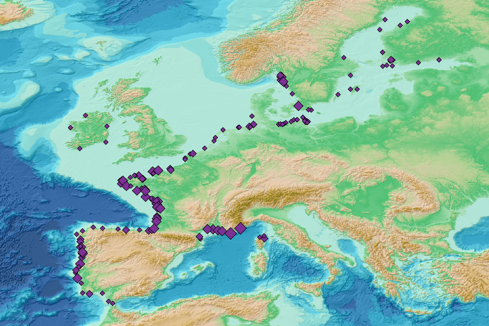
This visualization product displays the cigarette related items abundance of marine macro-litter (> 2.5cm) per beach per year from Marine Strategy Framework Directive (MSFD) monitoring surveys without UNEP-MARLIN data. EMODnet Chemistry included the collection of marine litter in its 3rd phase. Since the beginning of 2018, data of beach litter have been gathered and processed in the EMODnet Chemistry Marine Litter Database (MLDB). The harmonization of all the data has been the most challenging task considering the heterogeneity of the data sources, sampling protocols and reference lists used on a European scale. Preliminary processings were necessary to harmonize all the data: - Exclusion of OSPAR 1000 protocol: in order to follow the approach of OSPAR that it is not including these data anymore in the monitoring; - Selection of MSFD surveys only (exclusion of other monitoring, cleaning and research operations); - Exclusion of beaches without coordinates; - Selection of cigarette related items only. The list of selected items is attached to this metadata. This list was created using EU Marine Beach Litter Baselines, the European Threshold Value for Macro Litter on Coastlines and the Joint list of litter categories for marine macro-litter monitoring from JRC (these three documents are attached to this metadata); - Exclusion of surveys referring to the UNEP-MARLIN list: the UNEP-MARLIN protocol differs from the other types of monitoring in that cigarette butts are surveyed in a 10m square. To avoid comparing abundances from very different protocols, the choice has been made to distinguish in two maps the cigarette related items results associated with the UNEP-MARLIN list from the others; - Normalization of survey lengths to 100m & 1 survey / year: in some case, the survey length was not exactly 100m, so in order to be able to compare the abundance of litter from different beaches a normalization is applied using this formula: Number of cigarette related items of the survey (normalized by 100 m) = Number of cigarette related items of the survey x (100 / survey length) Then, this normalized number of cigarette related items is summed to obtain the total normalized number of cigarette related items for each survey. Finally, the median abundance of cigarette related items for each beach and year is calculated from these normalized abundances of cigarette related items per survey. Sometimes the survey length was null or equal to 0. Assuming that the MSFD protocol has been applied, the length has been set at 100m in these cases. Percentiles 50, 75, 95 & 99 have been calculated taking into account cigarette related items from MSFD monitoring data (excluding UNEP-MARLIN protocol) for all years. More information is available in the attached documents. Warning: the absence of data on the map does not necessarily mean that they do not exist, but that no information has been entered in the Marine Litter Database for this area.